1. Overview
Irradiation raises the yield strength of steel and lowers its fracture toughness. For a large plate with a central through-thickness crack, how does the assessment point drift on the Failure Assessment Diagram (FAD) over 20 years of service? Which year and which stress level is the most critical? How is the safety factor read? This post answers these three questions with the FITNET Basic Training Package example, assessed per BS 7910:2019 Clause 7; the BS 7910 Clause 7 fracture assessment calculator is only the entry point for trying it yourself, and its use is described in A Concise Guide to BS 7910 Fracture Assessment .
The example: the FITNET Basic Training Package example Plate under neutronic irradiation. Authors: F. Gutiérrez-Solana, S. Cicero, J. A. Álvarez, R. Lacalle (University of Cantabria). The package was issued with the FITNET FFS Procedure (MK7, 2006).
Methods on the two sides: the source uses $K_I=\sigma\sqrt{\pi a}$ and $L_r=\sigma/\sigma_Y$. mechCalc uses the BS 7910 Annex M through-thickness crack solution and the Annex P reference stress solution. For an infinitely wide plate the two reduce to the same formulas, so any difference between the two sides should come only from the number of decimals in the source.
Conclusion first:
- The 12 assessment points: Where the source gives three decimals, the difference is at most 0.002. Where the source gives only two decimals, the difference is within 0.01. All differences come from rounding in the source.
- Most critical case: year 20, 350 MPa.
- Safety factor of that point: mechCalc gives a reserve factor on load $F_{load}=1.19$; the source reads 1.2 from its chart with the ray method.
2. The Example
A large steel plate contains a central through-thickness crack of length $2a=20$ mm. The working tensile stress has four levels: 50, 150, 250 and 350 MPa.
The plate is exposed to neutron irradiation. The material changes with time: yield strength rises and fracture toughness falls. The source gives material data for five years:
| Irradiation time (years) | 0 | 5 | 10 | 15 | 20 |
|---|---|---|---|---|---|
| Yield strength $\sigma_Y$ [MPa] | 500 | 510 | 540 | 565 | 585 |
| Fracture toughness $K_{Ic}$ [MPa·m$^{0.5}$] | 150 | 135 | 120 | 100 | 85 |
The source asks three questions:
- Plot the safety state at years 0, 10 and 20 on the FAD.
- Which case is the most critical?
- For how long is the safety factor greater than 1.2?
The source solution is short. For a large plate, the stress intensity factor is $K_I=\sigma\sqrt{\pi a}$. With a half-length $a=0.01$ m this gives $K_I=0.177\,\sigma$. The fracture ratio is $K_r=K_I/K_{Ic}$ and the load ratio is $L_r=\sigma/\sigma_Y$. The 12 points are plotted on the standard FAD. The safety factor comes from the ray method: draw a ray from the origin O through the assessment point A; it meets the failure assessment line at B; then $\mathrm{S.F.}=OB/OA$.
The physical picture in one sentence: irradiation raises $\sigma_Y$ and lowers $K_{Ic}$. So $L_r$ gets smaller and $K_r$ gets larger. The assessment point drifts up and to the left, toward the brittle-fracture part of the curve.
3. Calculation with mechCalc
3.1 Input data
The most critical point (year 20, 350 MPa) is used as the example.
| Parameter | Value | Note |
|---|---|---|
| Geometry group / flaw type | Flat plate / through-thickness crack | Annex M.3.1 / P.4.1 |
| Crack depth $a$ | 10 mm | For a through-thickness crack, $a$ is the half-length |
| Thickness $B$ | 25 mm | Any value. A through-thickness crack under pure tension does not use $B$ in the formulas |
| Component width $W$ | 100000 mm | Stands in for an infinitely wide plate |
| Primary membrane stress $P_m$ | 350 MPa | Working tensile stress |
| Primary bending stress $P_b$ | 0 | Pure tension |
| Secondary load | none | The example has no residual stress |
| Yield strength $\sigma_Y$ | 585 MPa | Year 20 |
| Tensile strength $\sigma_U$ | 819 MPa | Not given in the source; taken as $1.4\sigma_Y$ |
| Young’s modulus $E$ | 210 GPa | Not given in the source; typical value for carbon steel |
| Fracture toughness $K_{mat}$ | 85 MPa·m$^{0.5}$ | $K_{Ic}$ at year 20 |
| FAD option | Option 1 | Standard curve |
| Source of plasticity interaction $\rho$ | zero | No secondary stress |
Two quantities are not given in the source. Here is what they do:
- $E$ only enters the shape parameter of the failure assessment line, $\mu=\min(0.001E/\sigma_Y,\,0.6)$. It does not change the coordinates of the assessment point. With $E$ = 200 or 210 GPa, $f(L_r)$ differs by only 0.0005.
- $\sigma_U$ only affects the part of the curve with $L_r>1$ and the cut-off value $L_{r,\max}$. All points in this example have $L_r<0.71$, so they are not affected.
3.2 Try it yourself: entering it in the calculator
One click: open this example in the calculator . The inputs are filled in for you; the steps below are for checking or entering them by hand.
- Assessment Option (FAD): keep FAD option 1.
- 1. Crack / Flaw Type: set Geometry to “Flat Plate” and Flaw to “Through-thickness (M.3.1 / P.4.1)”. Enter crack depth 10.
- 2. Component Geometry: thickness 25, component width 100000.
- 3. Stress & Polynomial Coefficients: primary membrane stress 350, primary bending stress 0. Set “Secondary (residual/thermal) load” to “None (no secondary stress)”.
- 5. Material: yield strength 585, tensile strength 819, elastic modulus 210.
- 6. Fracture Toughness: enter 85 for the fracture toughness (in the first version of the calculator, $K_{mat}$ can only be entered directly).
- 7. Analysis Type & Plasticity Interaction: set “Plasticity Interaction ($\rho$) Source” to “Zero (no secondary stress only)”. The first version of the calculator does initiation analysis only, so this card no longer shows an analysis type.
- Click Run Calculation.
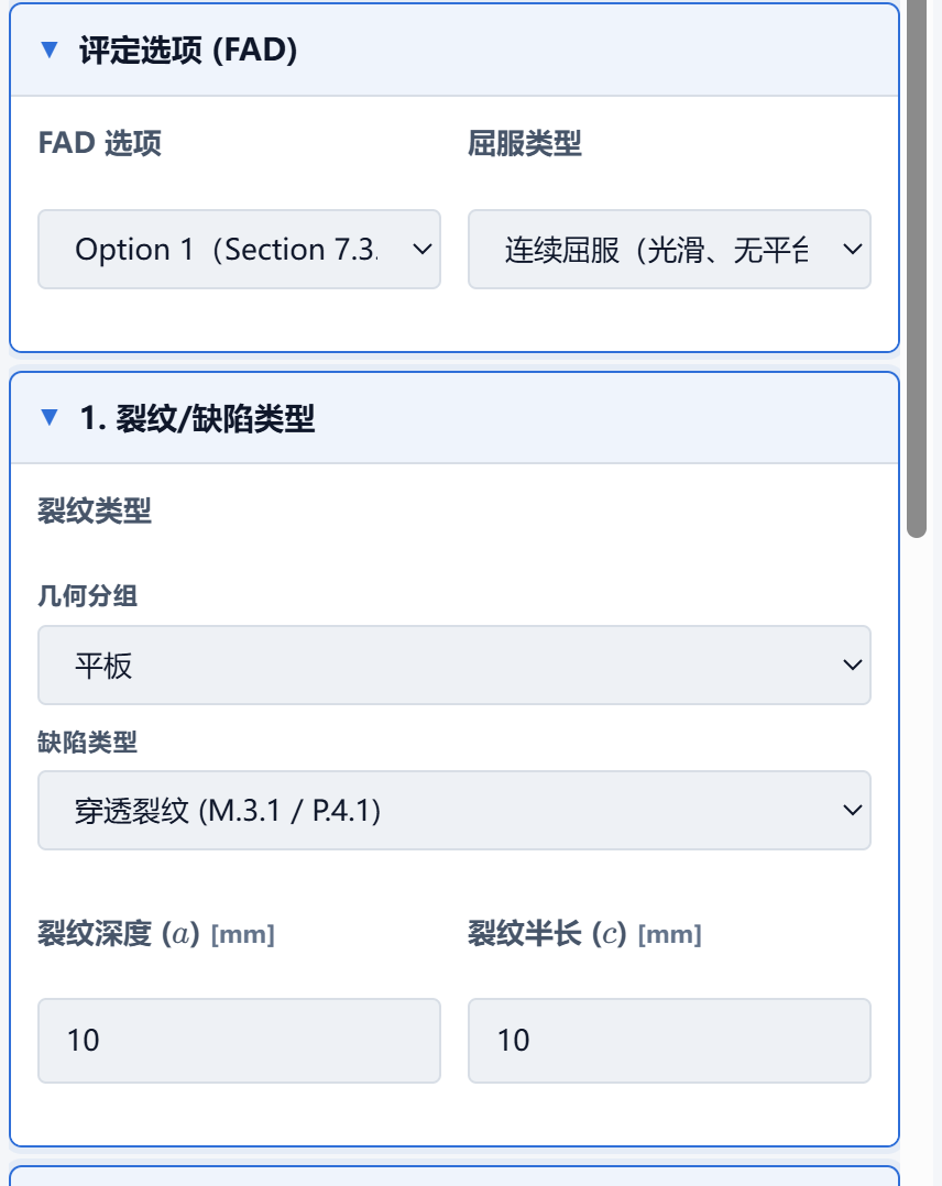 Figure 1: Assessment option and flaw type. The verification example drop-down has loaded this example; flat plate, through-thickness crack, crack depth a=10 mm (for a through-thickness crack, a is the half-length, and no half-length c is entered).
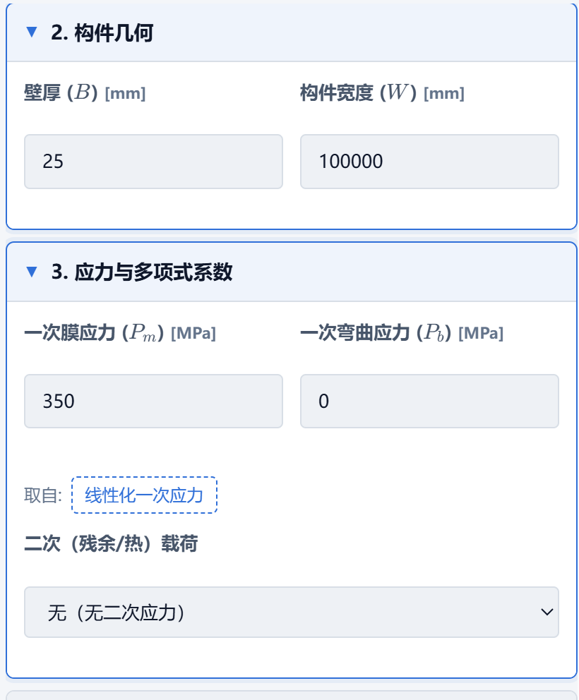 Figure 2: Component geometry and stress. W=100000 mm stands in for an infinitely wide plate; only the primary membrane stress of 350 MPa is entered, and the secondary (residual/thermal) load is set to None.
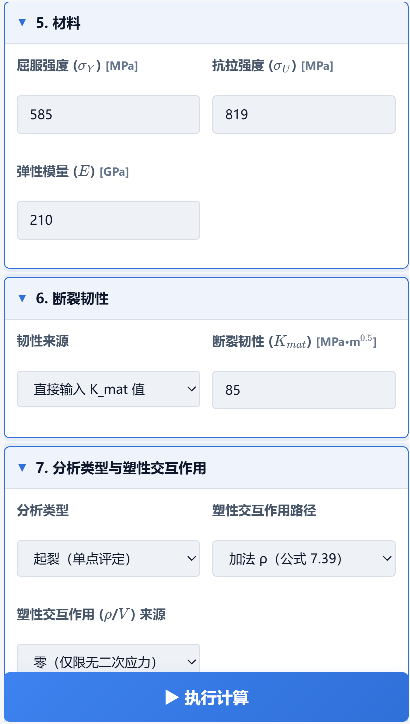 Figure 3: Material, fracture toughness and plasticity interaction. Material at year 20: σ_Y=585 MPa, K_mat=85 MPa·m^0.5; ρ source set to Zero.
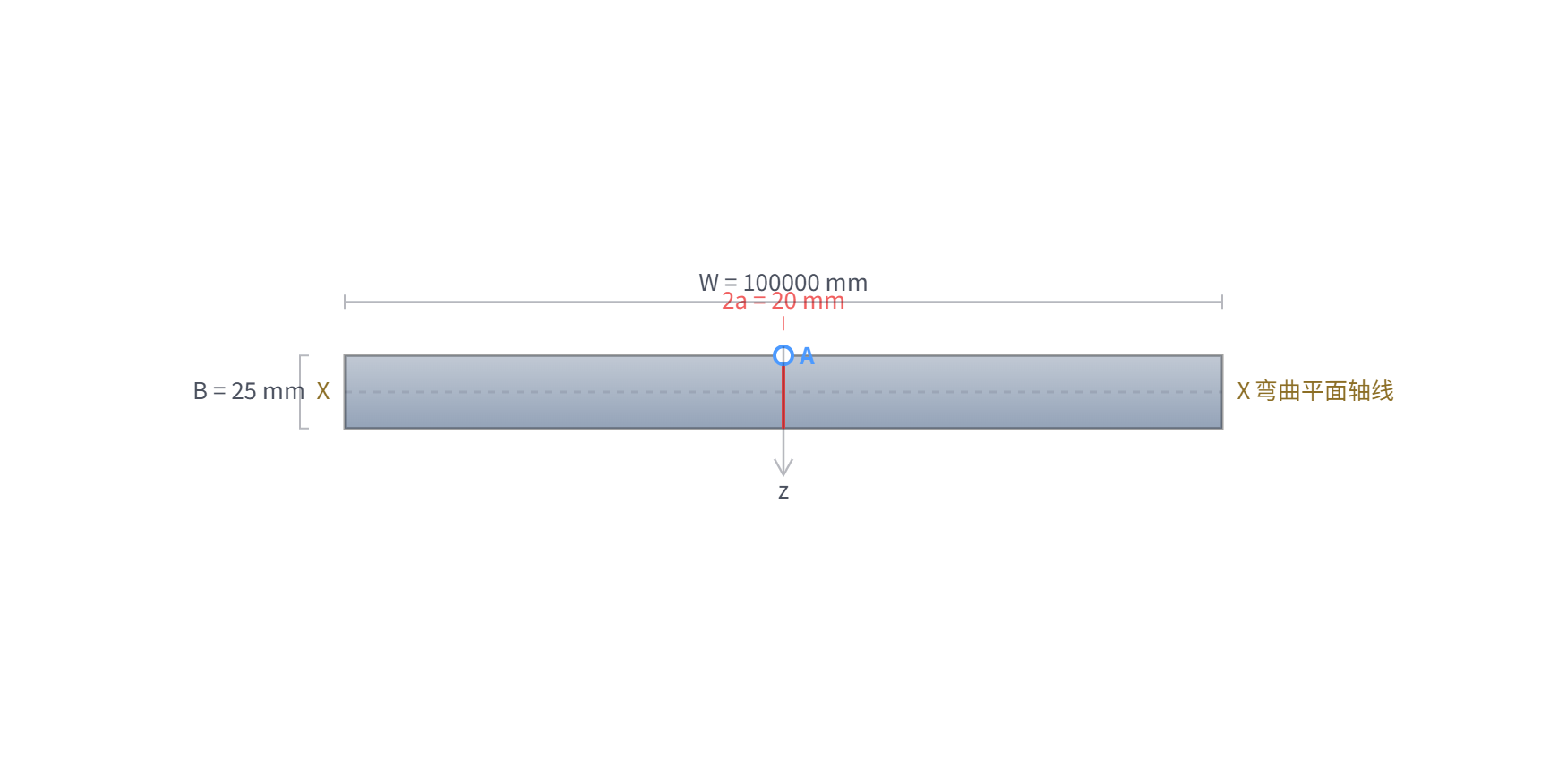 Figure 4: Crack geometry shown on the calculator’s Schematic tab. Central through-thickness crack, full length 2a=20 mm.
3.3 Calculation steps
The calculator assembles the assessment point in the order of Clause 7. Each step shows the formula and the substituted values.
Step 1: primary stress intensity factor (BS 7910:2019, Annex M, Eq. M.1; through-thickness crack in a plate, M.3.1)
$$K_I^P = (Y\sigma)\sqrt{\pi a}$$For a through-thickness crack in a plate: $M=1$, $M_m=1$, and the finite-width correction is $f_w=[\sec(\pi a/W)]^{0.5}$ (Eq. M.8). For very large $W$, $f_w=1$. So
$$K_I^P = 350\times\sqrt{\pi\times 0.010} = 62.04\ \mathrm{MPa\cdot m^{0.5}}$$Step 2: reference stress and load ratio (BS 7910:2019, Annex P, P.4.1, Eq. P.3; §7.3.7, Eq. 7.40)
$$\sigma_{ref}=\frac{P_b+\sqrt{P_b^2+9P_m^2}}{3\,(1-2a/W)}=\frac{3\times 350}{3\times(1-20/100000)}=350.07\ \mathrm{MPa}$$$$L_r=\frac{\sigma_{ref}}{\sigma_Y}=\frac{350.07}{585}=0.5984$$Step 3: fracture ratio (§7.3.6, Eq. 7.39)
$$K_r=\frac{K_I^P+K_I^S}{K_{mat}}+\rho=\frac{62.036+0}{85}+0=0.7298$$Step 4: failure assessment line (§7.3.3, Eq. 7.26, the $L_r\le 1$ part)
$$f(L_r)=\left(1+\tfrac{1}{2}L_r^2\right)^{-1/2}\left[0.3+0.7\,e^{-\mu L_r^6}\right]$$$\mu=\min(0.001\times 210000/585,\ 0.6)=0.359$. Substituting $L_r=0.5984$ gives $f(L_r)=0.9104$.
Step 5: verdict, margin and reserve factor
- $K_r=0.7298
- $L_r=0.5984
- Reserve factor on load $F_{load}=1.186$: the factor by which the primary load can be scaled until the assessment point reaches the FAL. The calculator finds it by a numerical root search. Here there is primary load only, so $K_r$ and $L_r$ are both proportional to the load, and the point moves along a straight line through the origin as the load grows. So $F_{load}$ is the same quantity as the $OB/OA$ of the source’s graphical method. This graphical method may be used to find the load factor for an initiation analysis under a single primary load (BS 7910:2019+C1:2025, N.2.4.6, Figure N.3).
- Margin on $K_r$, $F_{Kr}=f(L_r)/K_r=1.247$: the ratio measured up the vertical axis to the FAL, at fixed $L_r$.
- $L_r=0.5984
3.4 Results
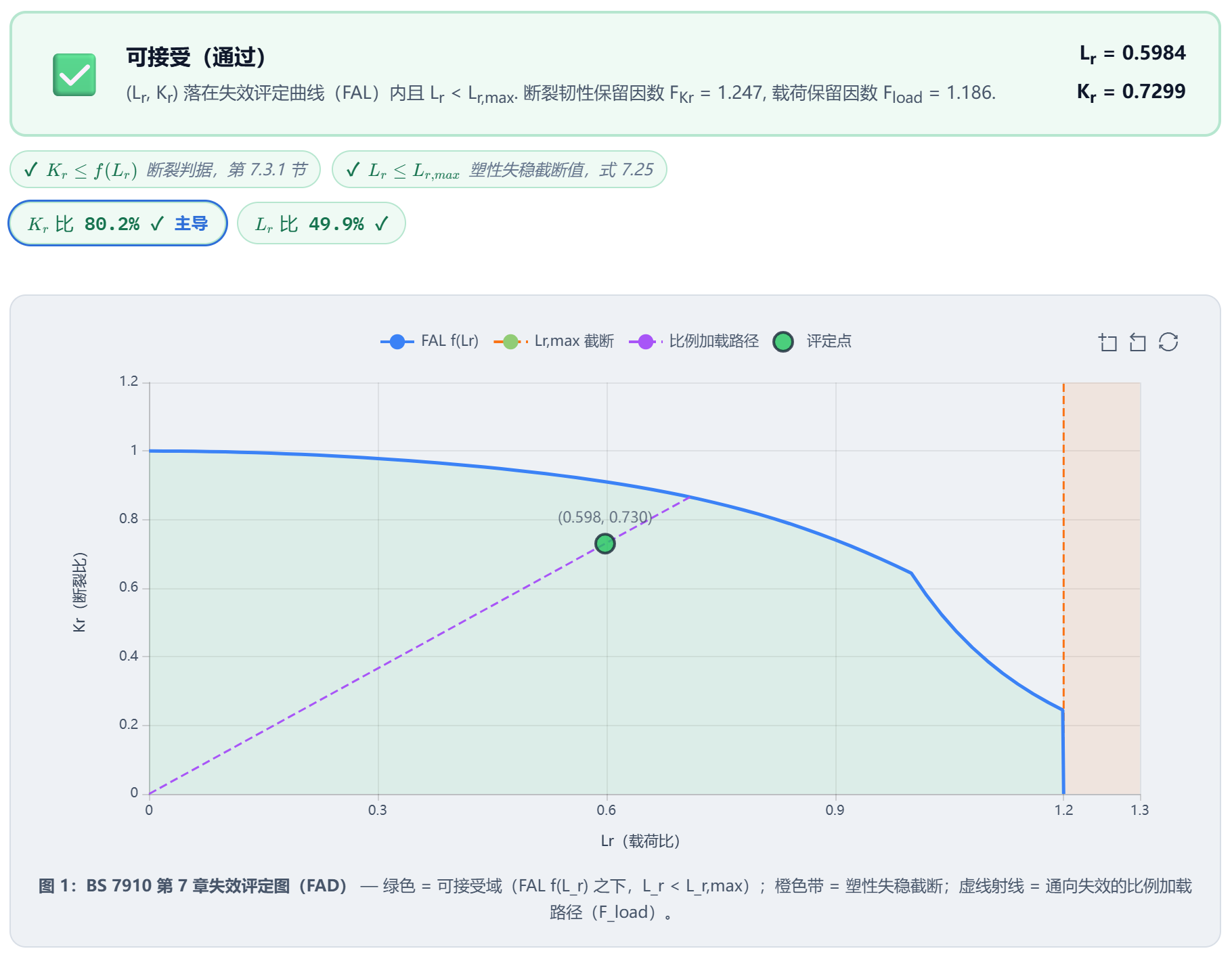 Figure 5: Result for year 20, 350 MPa. Verdict: acceptable. The assessment point (0.598, 0.730) lies inside the failure assessment line. The dotted vertical line is the margin on K_r, F_Kr=1.247; the dashed line runs from the assessment point to where it reaches the FAL when the primary load is scaled by F_load=1.186.
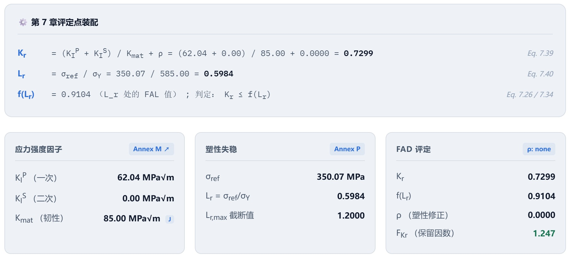 Figure 6: Assembly of the assessment point and intermediate quantities. K_I^P=62.04, σ_ref=350.07, f(L_r)=0.9104, margin on K_r F_Kr=1.247, reserve factor on load F_load=1.186.
3.5 The other assessment points
For the other points, only three inputs change: $P_m$, $\sigma_Y$ and $K_{mat}$. Everything else stays as it is. The table below sums up the results of all 20 points (5 years × 4 stress levels). The source gives only years 0, 10 and 20; years 5 and 15 were added by mechCalc.
| $\sigma$ [MPa] | Year | $K_I^P$ | $L_r$ | $K_r$ | $f(L_r)$ | $F_{load}$ | Verdict |
|---|---|---|---|---|---|---|---|
| 50 | 0 | 8.86 | 0.1000 | 0.0591 | 0.9975 | 10.08 | Acceptable |
| 50 | 5 | 8.86 | 0.0981 | 0.0656 | 0.9976 | 9.93 | Acceptable |
| 50 | 10 | 8.86 | 0.0926 | 0.0739 | 0.9979 | 9.82 | Acceptable |
| 50 | 15 | 8.86 | 0.0885 | 0.0886 | 0.9980 | 9.13 | Acceptable |
| 50 | 20 | 8.86 | 0.0855 | 0.1043 | 0.9982 | 8.30 | Acceptable |
| 150 | 0 | 26.59 | 0.3001 | 0.1772 | 0.9780 | 3.36 | Acceptable |
| 150 | 5 | 26.59 | 0.2942 | 0.1969 | 0.9789 | 3.31 | Acceptable |
| 150 | 10 | 26.59 | 0.2778 | 0.2216 | 0.9811 | 3.27 | Acceptable |
| 150 | 15 | 26.59 | 0.2655 | 0.2659 | 0.9827 | 3.04 | Acceptable |
| 150 | 20 | 26.59 | 0.2565 | 0.3128 | 0.9839 | 2.77 | Acceptable |
| 250 | 0 | 44.31 | 0.5001 | 0.2954 | 0.9385 | 2.02 | Acceptable |
| 250 | 5 | 44.31 | 0.4903 | 0.3282 | 0.9411 | 1.99 | Acceptable |
| 250 | 10 | 44.31 | 0.4631 | 0.3693 | 0.9478 | 1.96 | Acceptable |
| 250 | 15 | 44.31 | 0.4426 | 0.4431 | 0.9525 | 1.83 | Acceptable |
| 250 | 20 | 44.31 | 0.4274 | 0.5213 | 0.9558 | 1.66 | Acceptable |
| 350 | 0 | 62.04 | 0.7001 | 0.4136 | 0.8659 | 1.44 | Acceptable |
| 350 | 5 | 62.04 | 0.6864 | 0.4595 | 0.8731 | 1.42 | Acceptable |
| 350 | 10 | 62.04 | 0.6483 | 0.5170 | 0.8909 | 1.40 | Acceptable |
| 350 | 15 | 62.04 | 0.6196 | 0.6204 | 0.9026 | 1.30 | Acceptable |
| 350 | 20 | 62.04 | 0.5984 | 0.7298 | 0.9104 | 1.19 | Acceptable |
$K_I^P$ is in MPa·m$^{0.5}$.
Plotting all 20 points on one FAD shows the drift at a glance:
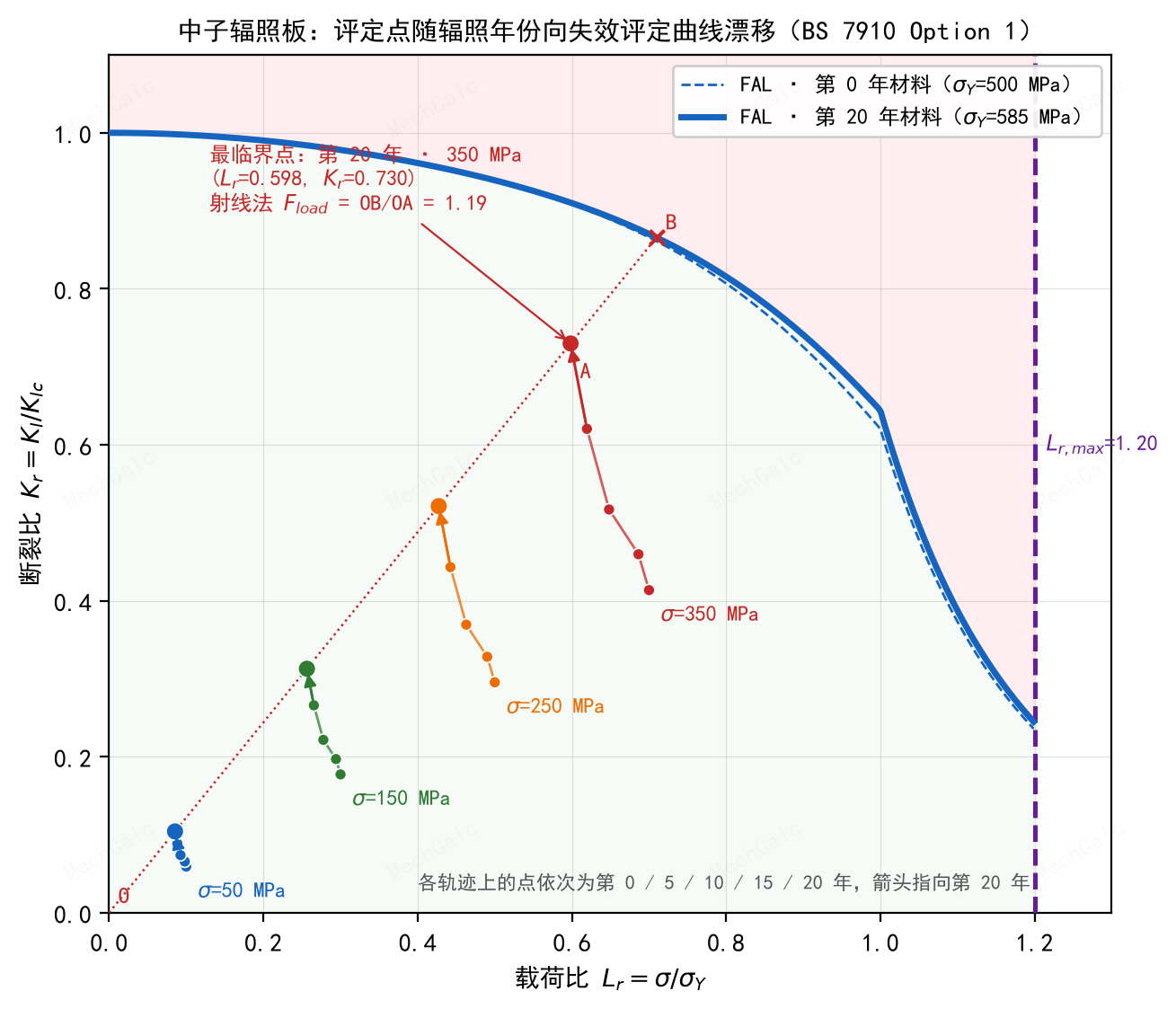 Figure 7: Drift of the 20 assessment points. The four paths belong to the four stress levels; each runs from year 0 to year 20. The higher the stress, the closer the path gets to the curve. The most critical point A is at year 20, 350 MPa. With primary load only, A moves along a straight line through the origin to B on the FAL as the load grows; OB/OA=1.19, the same as F_load. The curve is drawn with mechCalc’s failure assessment line function. (labels in Chinese)
4. Comparison of the Example Results with mechCalc
4.1 The 12 assessment points
| $\sigma$ [MPa] | Year | Source $K_r$ | mechCalc $K_r$ | Source $L_r$ | mechCalc $L_r$ |
|---|---|---|---|---|---|
| 50 | 0 | 0.06 | 0.059 | 0.10 | 0.100 |
| 50 | 10 | 0.073 | 0.074 | 0.092 | 0.093 |
| 50 | 20 | 0.104 | 0.104 | 0.085 | 0.085 |
| 150 | 0 | 0.18 | 0.177 | 0.30 | 0.300 |
| 150 | 10 | 0.221 | 0.222 | 0.277 | 0.278 |
| 150 | 20 | 0.312 | 0.313 | 0.25 | 0.257 |
| 250 | 0 | 0.30 | 0.295 | 0.50 | 0.500 |
| 250 | 10 | 0.368 | 0.369 | 0.463 | 0.463 |
| 250 | 20 | 0.520 | 0.521 | 0.42 | 0.427 |
| 350 | 0 | 0.42 | 0.414 | 0.70 | 0.700 |
| 350 | 10 | 0.516 | 0.517 | 0.648 | 0.648 |
| 350 | 20 | 0.728 | 0.730 | 0.59 | 0.598 |
How to read this table:
- Where the source gives three decimals (the $K_r$ values at years 10 and 20, the $L_r$ values at year 10), the two sides differ by at most 0.002.
- Where the source gives only two decimals (all of year 0, and $L_r$ at year 20), the difference is within 0.01. The source’s $L_r$ at year 20 is truncated, not rounded (350/585=0.598 is written as 0.59).
- The source uses $K_I=0.177\sigma$. The exact value is $\sqrt{\pi\times 0.01}=0.1772$. At 350 MPa, $K_I$ is 61.95 against 62.04, a difference of 0.15%.
- Same method, same formulas: the differences between the two sides come only from the number of decimals in the source.
4.2 The three questions of the source
| Question | Source answer | mechCalc |
|---|---|---|
| Which case is the most critical? | Year 20, 350 MPa | Same. At this point the $K_r$ ratio is 80.2%, the governing criterion |
| Safety factor at year 20 | $OB/OA=1.2$ (read from the chart) | $F_{load}=1.186$ (numerical solution) |
| How long is the safety factor greater than 1.2? | The first 20 years | 1.30 at year 15, 1.19 at year 20 |
The last row deserves a comment. The source reads 1.2 from its chart, so it says the safety factor stays above 1.2 for the first 20 years. mechCalc finds the reserve factor on load by a numerical root search and gets 1.19. The two differ by 1%, which is within chart-reading accuracy. If a factor strictly greater than 1.2 is required, the critical time lies between year 15 and year 20. This detail is hard to see in a hand-drawn chart.
4.3 What this example covers and what it does not
- It covers: the 12 assessment points, the most critical case, and the safety factor (the source’s ray-method $OB/OA$, which is mechCalc’s reserve factor on load $F_{load}$). $K_I$, $\sigma_{ref}$ and the assembly of the failure assessment line are all on the same basis as the source.
- What you must supply yourself: $E$ and $\sigma_U$, which the source does not give. As explained above, they do not change the assessment points of this example; their effect on $F_{load}$ is of the order of 0.001.
- Limit: the source has primary stress only. Secondary stress and the plasticity interaction correction $\rho$ are both zero in this example, so they are not involved here. For these quantities, see BS 7910 FAD Assessment: What Residual Stress Does, Seen Through a FITNET Case .
🧮 Online calculator: BS 7910 Clause 7 Fracture Assessment Calculator — Try it yourself: flat plate, through-thickness crack, a=10, W=100000, P_m=350, σ_Y=585, K_mat=85. You get L_r=0.598, K_r=0.730, F_load=1.19.
Verification manual for this calculator: BS 7910 Fracture Assessment Calculator verification manual