This is the first of four problems on the A533B-1 welded plate. The shared background, common method, and residual-stress profile for all four are set out in the overview post:
For the overview and method, see BS 7910 FAD Assessment: What Residual Stress Does, Seen Through a FITNET Case . This post focuses on one specimen and walks it through the calculator from input to reading the chart.
What this problem asks
LLAW = Low-$L_r$ + as-Welded: as-welded (no post-weld heat treatment), assessment temperature −120 ℃, low load ratio. Of the four specimens, it fractured at the lowest load (1.27 MN), with crack arrest afterwards. The low temperature drops the fracture toughness onto the lower shelf ($K_{mat}=37\ \mathrm{MPa\cdot m^{0.5}}$), while the full set of unrelaxed welding residual stresses still bears directly on the crack.
The aim here is to turn a qualitative statement — “welding residual stress is very damaging” — into a specific vertical-axis increment on the Failure Assessment Diagram (FAD).
The principle in brief: residual stress enters only K_r, not L_r
All four problems use the Option 1 (standard) Failure Assessment Diagram of BS 7910:2019 §7.3.3. The assessment-point coordinates:
$$ K_r = \frac{K_I^P + K_I^S}{K_{mat}} + \rho, \qquad L_r = \frac{\sigma_{ref}}{\sigma_Y} $$The Failure Assessment Line (FAL):
$$ f(L_r) = \begin{cases} \left(1 + \tfrac{1}{2}L_r^2\right)^{-1/2}\left[0.3 + 0.7\,e^{-\mu L_r^6}\right], & L_r \le 1 \\ f(L_r{=}1)\,L_r^{(N-1)/(2N)}, & 1 < L_r < L_{r,\max} \\ 0, & L_r \ge L_{r,\max} \end{cases} $$$$ \mu = \min\!\left(0.001\tfrac{E}{\sigma_Y},\ 0.6\right), \quad N = 0.3\left(1 - \tfrac{\sigma_Y}{\sigma_U}\right), \quad L_{r,\max} = \frac{\sigma_Y + \sigma_U}{2\sigma_Y} $$The three branches correspond to BS 7910:2019 §7.3.3 Eq. 7.26 ($L_r \le 1$, the brittle-fracture-governed branch), Eq. 7.27 ($1 < L_r < L_{r,\max}$, the elastic-plastic transition branch, where the curve bends down with the strain-hardening exponent $N$), and Eq. 7.28 ($L_r \ge L_{r,\max}$, plastic cut-off, where the curve drops to zero); the cut-off point $L_{r,\max}$ is given by Eq. 7.25. For this problem the assessment point sits at $L_r=0.367$, within the first branch, so the verdict below uses only Eq. 7.26.
The key engineering division of labour (BS 7910:2019, §7.3.6 / §7.3.7): welding residual stress is a secondary stress (a self-balancing field). It raises the vertical axis $K_r$ only and does not enter the horizontal axis $L_r$ — $L_r$ comes solely from the primary stress (here the bending stress of four-point bending), via the Annex P reference-stress solution. So the residual-stress contribution is simply the $K_I^S$ obtained by integrating the measured profile against the crack front with a weight function, entered directly and added into the numerator of $K_r$. For this problem the as-welded residual $K_I^S \approx 46\ \mathrm{MPa\cdot m^{0.5}}$ at the deepest point.
Both points of a semi-elliptical surface flaw are assessed: the calculator builds one assessment point at the deepest point and one at the surface point. Both points share the same $L_r$ (one $\sigma_{ref}$ per flaw); each has its own $K_r$. If either point lies on or outside the FAL, the flaw is not acceptable, and each reserve factor takes the smaller of the two points. This follows by analogy the BS 7910:2019+C1:2025 B.5.6 requirement to assess both the deepest point and the surface point (“If any of the points lie on or outside the locus, the flaw is unacceptable”; that sentence is written for tubular joints). So a directly entered $K_I^S$ also has two fields: 46 at the deepest point and 0 at the surface point. The surface value is 0 because integrating the same as-welded profile with Annex M.4.2 gives $K_I = -0.028\ \mathrm{MPa\cdot m^{0.5}}$ at the surface point (see the Annex M.4.2 post in this series ), and when $K_I^S<0$, both $K_I^S$ and $\rho$ are set to 0 (BS 7910:2019, §7.3.6).
Inputs at a glance
| Parameter | Value | Note |
|---|---|---|
| Flaw type | surface semi-elliptical (surface) | machined in the weld region |
| Crack depth $a_0$ / half-length $c_0$ | 19.4 / 87.5 mm | full length $2c_0=175$ mm |
| Plate thickness $B=t$ / width $W$ | 71 / 600 mm | |
| Primary membrane $P_m$ / bending $P_b$ | 0 / 245 MPa | pure bending (converted from the 1.27 MN fracture load) |
| Yield $\sigma_Y$ / tensile $\sigma_U$ | 618 / 791 MPa | base-metal properties |
| Elastic modulus $E$ | 210 GPa | |
| Fracture toughness $K_{mat}$ | 37 MPa·m$^{0.5}$ | as-welded weld @ −120 ℃, lower shelf |
| Residual $K_I^S$ (direct entry, deepest / surface point) | 46 / 0 MPa·m$^{0.5}$ | weight-function integration of the measured profile; the surface value is negative, so 0 is used |
Try it yourself: entering it in the calculator
One click: open this example in the calculator . The inputs are filled in for you. You can also pick “FITNET A533B residual stress — LLAW (as-welded, low load)” from the “Verification examples” list at the top of the calculator. The steps below are for checking or entering the inputs by hand.
mechCalc’s Fracture Assessment Calculator groups the inputs into cards, and the very first card is “Assessment Option (FAD)” — choose the method first, then fill in the data:
- Assessment Option (FAD): set “FAD Option” to
Option 1 (Section 7.3.3)(it is the default) and leave “Yielding Type” at the default continuous yielding. - 1. Crack / Flaw Type: set “Geometry” to
Flat Plateand the flaw type toSurface semi-elliptical (M.4.1 / P.5.1); enter crack depth 19.4 and crack half-length 87.5. - 2. Component Geometry: wall thickness 71, component width 600; leave the bending restraint at the default (restrained, Eq. P.9).
- 3. Stress & Polynomial Coefficients: primary membrane stress $P_m=0$, primary bending stress $P_b=245$; set “Secondary (residual/thermal) load” to
Enter K_I^S directly, then enter 46 in “Secondary SIF ($K_I^S$, direct)” (deepest point) and 0 in “Secondary SIF at Surface Point ($K_I^S$, direct)”. - 4. Stress Magnifiers (Weld Toe / Misalignment): leave every factor at the default 1 (no weld toe, misalignment or large-scale structural stress raiser in this problem).
- 5. Material: yield strength 618, tensile strength 791, elastic modulus 210.
- 6. Fracture Toughness: enter $K_{mat}=37$.
- 7. Analysis Type & Plasticity Interaction: this card now has only “Plasticity Interaction ($\rho$) Source”. Leave it at
Annex R (calculated) — default; the calculator finds $\rho$ at each of the two points. When a secondary stress is present, $\rho$ must be included and must not be set to zero, otherwise $K_r$ is non-conservative (BS 7910:2019, §7.3.6 sets $\rho$ to zero only when $K_I^S<0$).
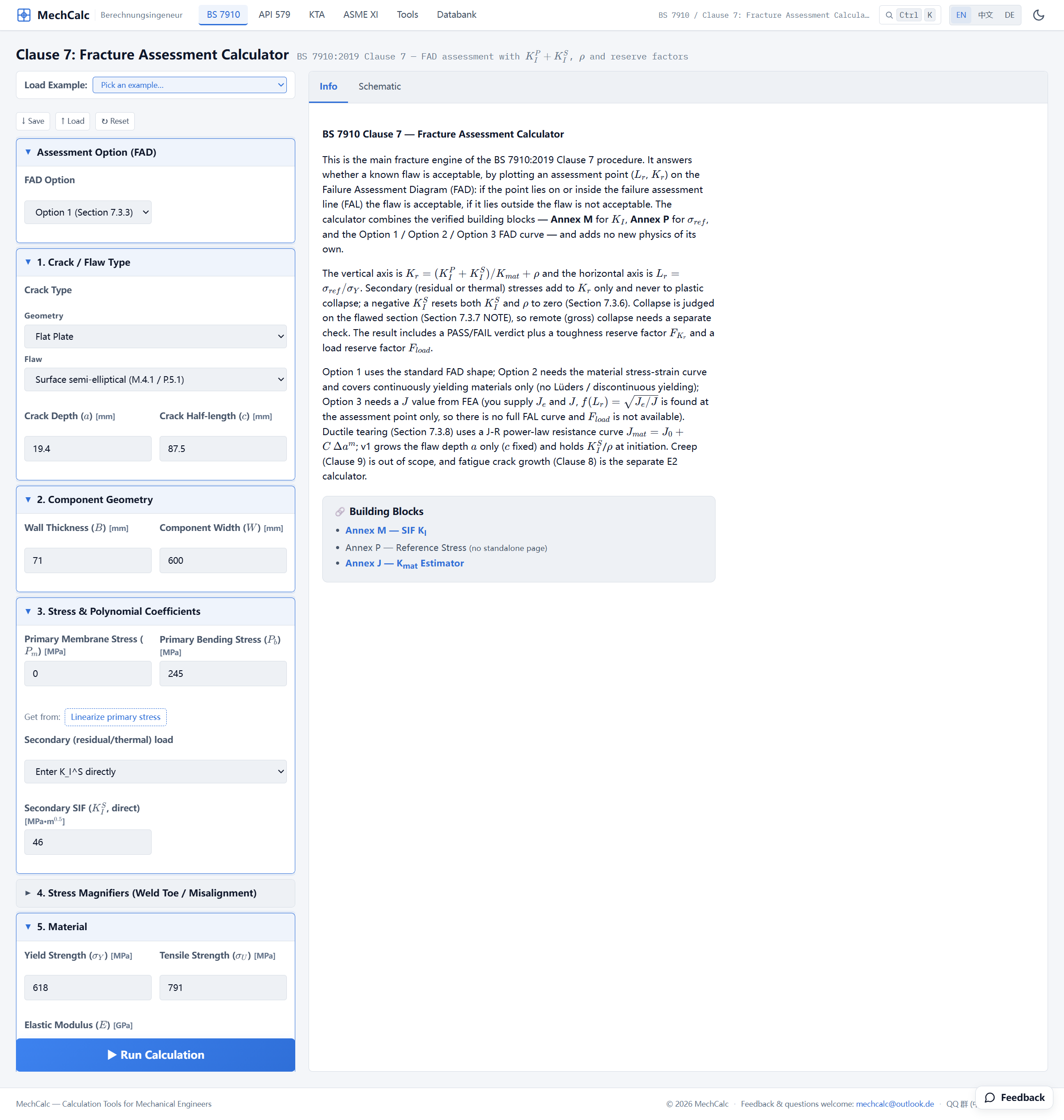 Figure 1: LLAW inputs in the Fracture Assessment Calculator. The top card “Assessment Option (FAD)” selects Option 1; the primary stress is bending only at 245 MPa; the welding residual stress enters the secondary channel as a directly entered K_I^S, 46 at the deepest point and 0 at the surface point.
Once everything is filled in, click Run Calculation.
Results
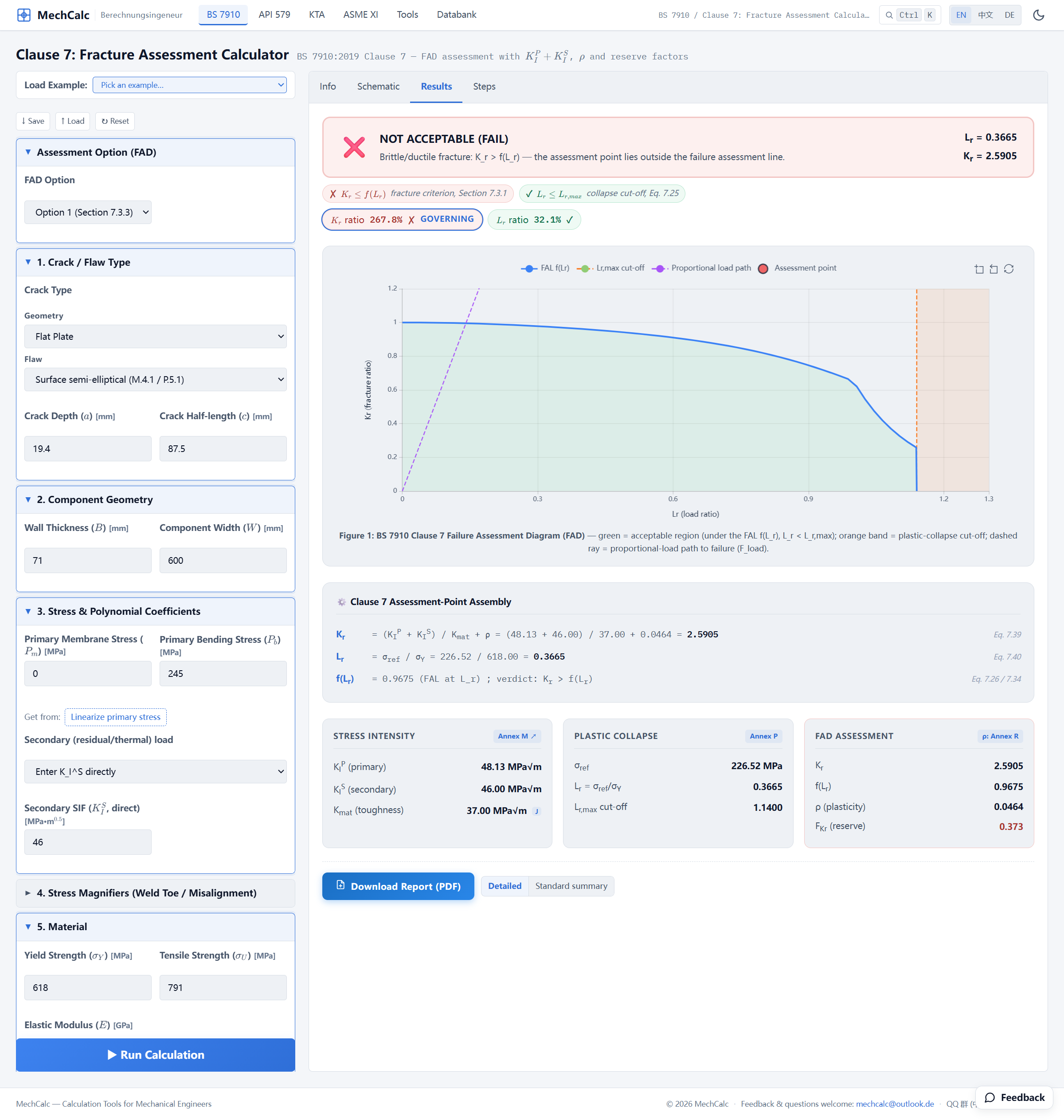 Figure 2: LLAW results. The banner says NOT ACCEPTABLE (brittle/ductile fracture): L_r=0.3665, K_r=2.5905 at the deepest point and 0.9150 at the surface point. On the FAD, the circle is the deepest point and the diamond is the surface point: the deepest point lies far outside the Failure Assessment Line, the surface point lies inside it. The two-point table below lists K_I^P, K_I^S, ρ, K_r and the verdict at both points.
The two assessment points and intermediate quantities the calculator builds via the Clause 7 procedure:
| Quantity | Deepest point | Surface point | Source |
|---|---|---|---|
| Primary stress intensity factor $K_I^P$ [MPa·m$^{0.5}$] | 48.13 | 33.86 | Annex M semi-elliptical surface-flaw solution |
| Secondary stress intensity factor $K_I^S$ [MPa·m$^{0.5}$] | 46.00 | 0 | direct entry (integration of the measured profile) |
| Plasticity interaction $\rho$ | 0.046 | 0 | Annex R |
| Vertical coordinate $K_r$ | 2.59 | 0.915 | $(K_I^P+K_I^S)/K_{mat}+\rho$ |
| Reference stress $\sigma_{ref}$ | 226.5 MPa (both points) | Annex P limit load | |
| Horizontal coordinate $L_r$ | 0.367 (both points) | $\sigma_{ref}/\sigma_Y$ | |
| FAL height $f(L_r)$ | 0.9675 | Eq. 7.26 | |
| Verdict at this point | not acceptable (fracture) | acceptable | $K_r$ against $f(L_r)$ |
| Verdict for the flaw | not acceptable (brittle fracture governing) | not acceptable if either point is not acceptable |
Reading the result
Start with the deepest point, which governs. Break $K_r$ apart and it becomes obvious: the numerator $K_I^P + K_I^S = 48.13 + 46 = 94.13$, of which the residual-stress term alone accounts for nearly half. If this were a piece of base metal with no residual stress ($K_I^S=0$), the deepest-point $K_r$ would land near $48.13/37 \approx 1.30$; the welding residual stress pushes it to 2.59 — almost double.
The deepest point $(0.367,\ 2.59)$ lies far beyond the Failure Assessment Line: at the same horizontal coordinate the FAL height is $f(L_r)=0.9675$, and $K_r$ is 2.7 times that. The ratio $f(L_r)/K_r=0.373$ is the margin on $K_r$, $F_{Kr}$, that the calculator reports (from the deepest point); a value below 1 means not acceptable. At the surface point $K_I^P$ is smaller and the residual term is 0, so $K_r=0.915$ lies inside the curve. But in a two-point assessment one unacceptable point is enough: the flawed structure is judged not acceptable. This matches the test: LLAW fractured at the lowest load. The main force driving it past the critical line is the residual stress intensity factor of 46 MPa·m$^{0.5}$ at the deepest point.
Why the reserve factor on load shows “—”: the reserve factor on load $F_{load}$ is the factor by which the primary load must be scaled (up or down) until the assessment point just reaches the FAL; the secondary stress does not change with the load (the calculator finds it as a root, following the load-factor approach of BS 7910:2019+C1:2025 Annex N.2.4.6, Figure N.3). At the deepest point of this problem, even with the primary load reduced to zero, $K_r$ is still at least $K_I^S/K_{mat}=46/37\approx1.24$, above the FAL height of 1.0 at $L_r=0$. The point stays outside the curve for any factor, so no such factor exists and the calculator shows “—” for the deepest point. This result says something on its own: the as-welded residual stress alone is enough to make this flaw not acceptable at −120 ℃. The surface point does have values ($F_{Kr}=1.057$, $F_{load}=1.054$), but the flaw is governed by the deepest point.
Comparison with the FITNET result
This problem also shows how two assessment procedures compare. Here are the results above set against the FITNET original (FITNET FFS Procedure MK7 (2006), Vol. II §13.2.5, Table 13.10), term by term. The mechCalc column is the governing deepest point:
| Quantity | mechCalc (deepest point) | FITNET original | Difference |
|---|---|---|---|
| Primary $K_I^P$ [MPa·m$^{0.5}$] | 48.13 | — | — |
| Secondary $K_I^S$ [MPa·m$^{0.5}$] | 46.0 | 46 | same source |
| Load ratio $L_r$ | 0.367 | 0.36 | +1.9% |
| Fracture ratio $K_r$ | 2.59 | 2.58 | +0.4% |
Note: the FITNET original (Vol. II §13.2.5, Table 13.10) lists only $K_r$ and $L_r$, not $K_I^P$, so the FITNET column shows “—”.
In the low-$L_r$, brittle-fracture-governed region — the very range that matters most to this test series — the two implementations agree almost digit for digit: $K_r$ differs by only 0.4% and $L_r$ by 1.9%. Bear in mind that the primary SIF and limit load on each side come from different analytical solutions (FITNET uses Sharples & Clayton / Sattari-Far, mechCalc uses BS 7910 Annex M / Annex P), and only the residual $K_I^S$ is taken from the same measured profile. Agreement this close shows that, in the low-$L_r$ region, the difference between the two sets of SIF and limit-load solutions has little effect on the assessment point ($K_r$ differs by 0.4%, $L_r$ by 1.9%); the position of the point is set mainly by the residual $K_I^S$ and the toughness.
Source: the FITNET project’s Case Studies for Fracture, case “A533B-1 Steel Residual Stress Experiments”; original test report C C France, J K Sharples & C Wignall, AEA Technology Report AEAT-4236 (SINTAP/TASK4/AEAT18, 1998). The LLAW fracture load of 1.27 MN, the crack arrest and the assessment inputs are in FITNET FFS Procedure MK7 (2006), Vol. II §13.2.5, Tables 13.9 / 13.10.
Next problem preview: same temperature, same region, same measured residual profile — the only variable is that post-weld heat treatment (PWHT) was applied, dropping the residual $K_I^S$ from 46 to 5. How far does the assessment point fall back? See Problem 2 LLHT .
🧮 Online calculator: BS 7910 Clause 7 Fracture Assessment Calculator — Try it yourself: pick Option 1, enter the inputs from the table above, enter K_I^S directly (46 at the deepest point, 0 at the surface point), and you get L_r=0.367 and K_r=2.59 at the deepest point.
Verification manual for this calculator: BS 7910 Fracture Assessment Calculator verification manual