In a BS 7910 fracture assessment most attention goes to flaw size, stress and toughness — but one thing hidden in the material is easy to miss: when this steel yields, does it pass smoothly into plasticity, or does it “catch, then let go” first? This small metallurgical detail grows a cliff in the failure assessment line near $L_r=1$ — get it wrong and you badly overestimate the safety margin. This article explains what yielding is, how continuous and discontinuous yielding differ, and how Option 1 and Option 2 each handle them.
If you are not yet comfortable with the horizontal axis $L_r$, the vertical axis $K_r$ and the dividing failure assessment line of the Failure Assessment Diagram (FAD), read the BS 7910 Fracture Assessment — A Concise Guide first; for an overview of how to choose among the three assessment options, see Clause 7’s Three Assessment Options: How to Choose Between Option 1 / 2 / 3 . This article covers one thing only: how the material’s yielding behaviour changes the shape of that FAL curve.
1. First, yielding: the step from “elastic” to “plastic”
Pull a metal bar and at first it acts like a spring — remove the load and it springs back. This is elastic deformation. But once the load passes a threshold, the bar keeps a permanent stretch that does not recover on unloading. That is yielding: the material crosses from recoverable elastic behaviour into unrecoverable plastic deformation. That threshold stress is the yield strength $\sigma_Y$.
Exactly which value you take for the yield strength depends on how “cleanly” the material yields:
- Some materials show a clear upper yield point $R_{eH}$ (the highest stress reached before the dislocations break free) and a lower yield strength $R_{eL}$ (the value the stress falls back to and settles at). For these, engineering practice takes the lower yield strength $R_{eL}$ as the yield strength — it is the more stable, safer value.
- Other materials yield “gradually”, with no clear yield point at all. For these a value is defined by convention: the stress that produces $0.2\%$ permanent plastic strain, written $0.2\%$ proof strength $R_{p0.2}$, is used as the nominal yield strength (BS 7910:2019, §7.1.3).
Those two ways of “yielding cleanly or not” are exactly the subject of this article — continuous versus discontinuous yielding.
2. Two yielding behaviours: continuous vs discontinuous
Draw the stress-strain curves of the two material types together and the difference is immediate:
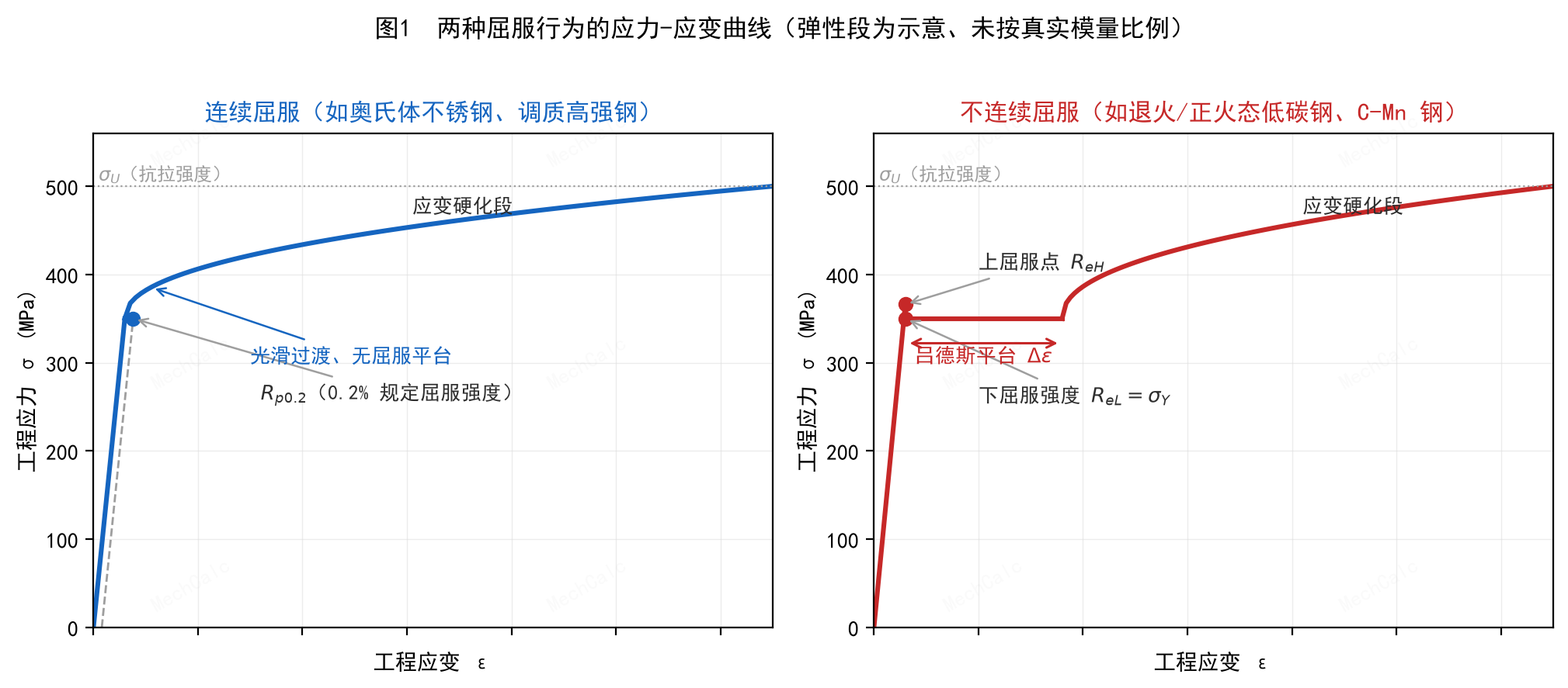
Figure 1: Stress-strain curves for the two yielding behaviours (the elastic part is schematic, not to true-modulus scale, so the yield details stay visible). Left: continuous yielding — past the yield region the curve rises smoothly with no plateau, and the yield strength is set by the 0.2% proof strength R_p0.2. Right: discontinuous yielding — the stress first peaks at the upper yield point R_eH, drops back to the lower yield strength R_eL, then runs along a Lüders plateau where the stress barely rises while the strain grows a lot (length Δε); strain hardening only begins once the plateau ends.
- Continuous yielding: the stress-strain curve passes smoothly, and past the yield point the stress keeps rising with strain (strain hardening) without any pause.
- Discontinuous yielding: after peaking at the upper yield point the stress falls back to the lower yield strength, and then a nearly flat plateau appears — the stress barely rises while the strain runs on. This plateau is the yield plateau or Lüders plateau, the large strain produced along it is the Lüders strain $\Delta\varepsilon$, and visible slanted slip bands — Lüders bands — appear on the surface.
Why is there a plateau? In microscopic terms: in low-carbon steel the carbon and nitrogen atoms gather around the dislocations and “pin” them like small locks (this cloud of atoms is the Cottrell atmosphere). To start deforming you must pull the dislocations free of the locks with a large force — this gives the raised upper yield point. But once free, the dislocations slide more easily through the lattice, so they move in large groups: macroscopically the load need not rise while the bar keeps stretching — the yield plateau. Only after most of these dislocations have run does the material enter the strain-hardening stage where force must rise again.
A note on terms: the rise of stress with strain after yield is called strain hardening in fracture mechanics (also “work hardening” in manufacturing); the strain-hardening exponent $n$ used later in Option 2 measures how strong it is.
3. Which materials are which?
Yielding type is set mainly by composition, heat treatment and processing history. Roughly:
Materials that tend to yield discontinuously (with a plateau):
- As-rolled or normalized low-carbon and C-Mn steels, especially rolled steel plate — the most typical group;
- carbon steels sensitive to strain aging, whose plateau is especially marked when they operate in the relevant temperature range.
Materials that tend to yield continuously (no plateau, smooth transition):
- austenitic stainless steels and aluminium alloys (their lattice does not readily form the Cottrell “locks”);
- quenched-and-tempered high-strength steels;
- cold-worked (cold-drawn, cold-rolled) steels — the dislocations were already pulled free during processing, so the yield plateau is used up in advance.
This is only an empirical tendency, not a rule. In §7.1.3.6, Table 7.4, BS 7910 gives detailed guidance on whether to assume a yield plateau in rolled steel plate, by yield strength range, process route, composition and heat treatment — when you have a specific grade and process, use that table (BS 7910:2019, §7.1.3.6, Table 7.4).
4. Not sure which? Be safe — assume “discontinuous”
In real work you cannot always get a full stress-strain curve for a given steel, nor be certain whether it has a plateau. What then?
The spirit of BS 7910 is: when data are insufficient and you cannot decide, the safe course is to [assume discontinuous yielding] (that is, assume a Lüders plateau exists). The standard even gives, for materials with $\sigma_Y < 1000\ \mathrm{N/mm^2}$, a direct estimate of the plateau length (BS 7910:2019, §7.1.3.6, Eq. (7.8)):
$$\Delta\varepsilon = 0.0375\,(1 - 0.001\,\sigma_Y)$$Why is “discontinuous” the conservative assumption? As Section 5 below shows, discontinuous yielding makes the failure assessment line drop like a cliff at $L_r=1$, pushing the allowed fracture ratio $K_r$ in that region very low. Assuming a plateau tightens the acceptance standard on purpose; conversely, treating a steel that actually has a plateau as continuous yielding overestimates the safety margin near $L_r\approx1$ and gives an unsafe result. Safety comes first — when unsure, it is better to assume the cliff is there.
When you have a specific grade and process: use Table 7.4
If you know the material’s yield strength range, process route, composition and heat treatment, BS 7910 gives a decision table for rolled steel plate (BS 7910:2019, §7.1.3.6, Table 7.4):
| Yield strength range (N/mm²) | Process route | Composition | Heat treatment | Assume yield plateau (discontinuous)? |
|---|---|---|---|---|
| $R_{eH}\le350$ | As-rolled | Conventional steels (e.g. BS EN 10025-2, no microalloy additions) | — | Yes |
| $R_{eH}\le350$ | As-rolled | Mo, Cr, Nb, Al or Ti present | — | (No) |
| $R_{eH}\le350$ | Normalized | BS EN 10025-2 type, no microalloy | Conventional normalizing | Yes |
| $R_{eH}\le350$ | Normalized | BS EN 10025-3 type, with microalloy | Conventional normalizing | Yes |
| $R_{eH}\le350$ | Controlled rolled | BS EN 10025-3 / 10025-4 | — | Yes |
| $R_{eH}>350$ | Controlled rolled | BS EN 10025-3 / 10025-4 | Light TMCR ($R_{eH}<400$) | Yes |
| $R_{eH}>350$ | Controlled rolled | BS EN 10025-3 / 10025-4 | Heavy TMCR ($R_{eH}>400$) | (Yes) |
| $R_{eH}\le500$ | Quenched & tempered | Mo or B present, with microalloy Cr/V/Nb/Ti | Heavy tempering (favours plateau) | Yes |
| $R_{eH}\le500$ | Quenched & tempered | Mo or B present, with microalloy | Light tempering (favours no plateau) | (Yes) |
| $R_{eH}\le500$ | Quenched & tempered | No Mo/B, but microalloy present (V especially strong) | Heavy tempering | (Yes) |
| $R_{eH}\le500$ | Quenched & tempered | No Mo/B, but microalloy present | Light tempering | (No) |
| $R_{p0.2}$ or $R_{eH}>500$ | Quenched & tempered | Mo or B present, with microalloy | Tempered to $R_{p0.2}<\sim690$ | (No) |
| $R_{p0.2}$ or $R_{eH}>500$ | Quenched & tempered | Mo or B present, with microalloy | Tempered to $R_{p0.2}>\sim690$ | No |
| $R_{p0.2}$ or $R_{eH}>500$ | Quenched & tempered | No Mo/B, but microalloy present | Tempered to $R_{p0.2}<\sim690$ | Yes |
| $R_{p0.2}$ or $R_{eH}>500$ | Quenched & tempered | No Mo/B, but microalloy present | Tempered to $R_{p0.2}\ge\sim690$ | (No) |
| $R_{p0.2}\le1000$ | As-quenched | All compositions | — | No |
A bracketed “(Yes)/(No)” in the table means the call is uncertain; then run a sensitivity analysis on whether the presence or absence of a plateau affects the assessment. Yield strength in the table is defined by the upper yield strength $R_{eH}$ (to harmonize with the relevant standards). TMCR means thermo-mechanical controlled rolling. Source: BS 7910:2019, §7.1.3.6, Table 7.4.
Now to the main point: how Option 1 and Option 2 each draw the two yielding behaviours into the FAL.
Before starting, keep in mind one thing that runs through the whole article: the assessment point $(L_r,\,K_r)$ is computed the same way regardless of yielding type; yielding type only changes the shape of the FAL curve $f(L_r)$. The horizontal $L_r=\sigma_{ref}/\sigma_Y$ and the vertical $K_r=(K_I^{\,p}+K_I^{\,s})/K_{mat}+\rho$ are computed as usual (BS 7910:2019, §7.3.6/§7.3.7).
5. Option 1’s way: swap the equations
Option 1 needs the least data (only $\sigma_Y$, $\sigma_U$, $E$), and its way of handling the two cases is direct — it keeps two sets of equations and switches by material.
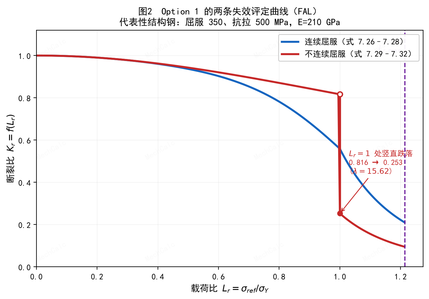
Figure 2: The two failure assessment lines Option 1 gives for the two yielding behaviours (representative structural steel σ_Y=350, σ_U=500 MPa, E=210 GPa). Blue: continuous yielding (Eq. 7.26–7.28). Red: discontinuous yielding (Eq. 7.29–7.32) — note it runs slightly above the blue line for Lr<1, yet drops vertically at Lr=1 from 0.816 to 0.253 and stays below the blue line afterwards. Both curves share the same plastic-collapse cut-off L_r,max at the right.
Continuous yielding uses this set (BS 7910:2019, §7.3.3, Eq. (7.26)–(7.28)):
$$f(L_r) = \left(1 + \tfrac{1}{2}L_r^2\right)^{-0.5}\left[\,0.3 + 0.7\exp\!\left(-\mu L_r^6\right)\right] \quad (L_r \le 1)$$$$\mu = \min\!\left(0.001\tfrac{E}{\sigma_Y},\; 0.6\right), \qquad N = 0.3\left(1 - \tfrac{\sigma_Y}{\sigma_U}\right)$$Discontinuous yielding switches to another set (BS 7910:2019, §7.3.3, Eq. (7.29)–(7.33)). There are two key differences:
- The $L_r<1$ branch becomes $f(L_r) = \left(1 + \tfrac{1}{2}L_r^2\right)^{-0.5}$ — the square-bracket term is gone (and with it $\mu$). So this branch sits slightly higher than the continuous curve.
- At $L_r=1$, $f$ drops vertically from its pre-plateau value to a lower one:
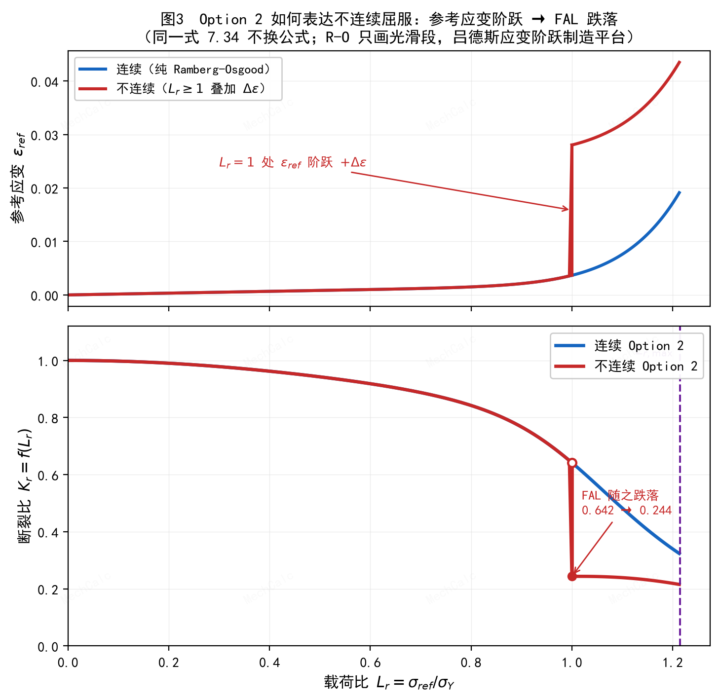
Why the vertical drop? At $L_r=1$ the reference stress just equals the yield strength, and the material runs a whole strain increment $\Delta\varepsilon$ along the yield plateau at nearly constant stress. The plastic deformation capacity of the flawed section is released at once, so the allowed $K_r$ drops like a cliff from its pre-plateau value to the post-plateau value. The parameter $\lambda$ measures the “total strain at the end of the plateau” relative to the “initial elastic yield strain” — the longer the plateau (the larger $\Delta\varepsilon$), the larger $\lambda$ and the deeper the drop (in Figure 2, $\lambda=15.6$ and $f$ falls straight from $0.816$ to $0.253$). After the drop, the $1 The right wall treats both alike: for either yielding type the horizontal axis ends at the plastic-collapse cut-off $L_{r,\max}=(\sigma_Y+\sigma_U)/2\sigma_Y$; beyond it $f$ is taken as zero — that is the boundary for overall plastic collapse of the flawed section (BS 7910:2019, §7.3.2, Eq. (7.25)). Option 2 is subtler. It builds the FAL from the material’s true stress-true strain curve and has just one equation (BS 7910:2019, §7.3.4, Eq. (7.34)) — it does not swap equations like Option 1: The magic is all in the reference strain $\varepsilon_{ref}$ — the true strain at the true stress $\sigma_{ref}=L_r\sigma_Y$, taken straight off the material’s real stress-strain curve. So: whenever the material’s stress-strain curve has a plateau at yield, $\varepsilon_{ref}$ jumps up sharply at $L_r=1$, and once that goes into the equation, $f(L_r)$ drops on its own. In other words, Option 2 needs no separate equation for discontinuous yielding — the input curve brings the cliff with it. So how is that plateau produced inside $\varepsilon_{ref}$? Here is a point easily misunderstood: MechCalc’s Option 2 fits the stress-strain curve with the Ramberg-Osgood (R-O) relation, and the R-O relation describes continuous yielding only (a smooth curve, as the standard states in §7.1.3.5 NOTE 1) — it cannot draw a plateau. So the standard’s approach is not to make R-O fit the plateau, but to add a Lüders-strain step on top of R-O by the “splicing” method of §7.1.3.6: R-O only draws the smooth shape of the elastic and strain-hardening parts; the $+\Delta\varepsilon$ step raises the strain by a jump at $L_r=1$ — this is the artificially reproduced Lüders plateau. Figure 3: How Option 2 expresses discontinuous yielding. Top — the reference strain ε_ref versus L_r: continuous (blue, pure Ramberg-Osgood) rises smoothly; discontinuous (red) adds the Lüders strain Δε at L_r=1, giving a vertical step. Bottom — the FAL after putting ε_ref into the same Eq. 7.34: the step in ε_ref makes f(L_r) drop from 0.642 to 0.244 at L_r=1. The equation did not change; the cliff comes from the input strain. Two paths, same destination: Option 1 in Figure 2 (the $\lambda$ drop) and Option 2 in Figure 3 (the $\varepsilon_{ref}$ step) come from completely different equations, yet both fall to a similar low value at $L_r=1$ (about $0.24\!\sim\!0.25$) — they describe the same physical plateau, so they should agree. This is also indirect confirmation that the splicing method is correct. An honest boundary: MechCalc’s Option 2 follows the “R-O approximate curve” route the standard permits, and the discontinuous handling above is its natural extension (an artificial splicing estimate). If you have a measured true stress-true strain curve (with a real plateau), a strict Option 2 should use that measured curve directly — that is more accurate and closer to the material’s real behaviour. The whole point in one sentence worth remembering: For a steel with a yield plateau, using the continuous-yielding equations overestimates the safety margin near $L_r\approx1$ — an unsafe error. For deciding which yielding type applies, see §7.1.3.6; when unsure, safely assume a plateau. Once the principle is clear, hands-on is quickest. In the online BS 7910 fracture assessment calculator, after choosing Option 1 or Option 2 you can switch the material’s yielding type (continuous / discontinuous): choose “discontinuous”, give the Lüders strain $\Delta\varepsilon$ (or let the program estimate it by Eq. 7.8), and watch the failure assessment line grow that cliff at $L_r=1$ and the assessment point’s margin tighten in real time. 🧮 在线计算器:BS 7910 Fracture Assessment Calculator — Under 'Assessment Option (FAD)' choose Option 1 or 2, switch continuous/discontinuous yielding, and watch in real time how the FAL drop at L_r=1 changes the verdict. The figures here are original MechCalc illustrations for teaching only; they do not replace the BS 7910 text. For engineering assessment use the current BS 7910:2019+A1:2020; the final decision on whether a flawed structure may remain in service must be confirmed by a qualified engineer with complete data and a sensitivity analysis.
6. Option 2’s way: one equation, and the “reference strain” grows the step itself
7. The cost of getting it wrong, and a one-page summary
Item
Continuous yielding
Discontinuous yielding (with Lüders plateau)
Stress-strain curve
Smooth transition, no plateau
Upper/lower yield point + yield plateau
Common materials
Austenitic stainless, aluminium alloy, Q&T high-strength steel, cold-worked steel
As-rolled/normalized low-carbon and C-Mn steel (especially rolled plate)
Yield strength taken as
$R_{p0.2}$
Lower yield strength $R_{eL}$
Option 1 handling
Eq. 7.26–7.28
Eq. 7.29–7.32, vertical drop at $L_r=1$ ($\lambda=1+E\Delta\varepsilon/R_{eL}$)
Option 2 handling
Pure R-O $\varepsilon_{ref}$
Add $\Delta\varepsilon$ to $\varepsilon_{ref}$ for $L_r\ge1$; same Eq. 7.34 drops on its own
When unsure
—
Be safe, assume this case
Try it online with MechCalc