The fracture assessment of a cracked structure watches two competing failure modes. This guide uses a single Failure Assessment Diagram (FAD) to weave together the assessment principle, the calculation chain, and the BS 7910 assessment steps into one clear storyline. By the end you should be able to see how an assessment point is computed and how it is judged acceptable or not.
Prologue: after a crack is found
When an in-service pressure vessel, pipe, or welded structure is inspected, crack-like flaws are often found. The question the engineer must answer is not “can this crack be used” — a crack is not something you “use” — but rather: can the structure that contains this flaw still operate safely under the current loads?
This is exactly what a fitness-for-service (FFS) assessment addresses. Clause 7 of BS 7910:2019 covers its most central piece — the fracture assessment: deciding whether a flaw of known size is acceptable under the given loads and material.
Ordinary strength design (“working stress < allowable stress”) breaks down here, because in linear-elastic theory the stress at a crack tip goes to infinity and cannot be compared with an allowable stress at all. Fracture mechanics uses a different language to answer the question.
1. A tug-of-war between two failure modes
A cracked structure can fail along two very different paths (BS 7910:2019, §7.1.1):
- Brittle fracture: the driving force at the crack tip exceeds the material’s fracture toughness, and the crack grows suddenly and rapidly, with almost no warning. Low temperature, high strength, and thick sections make this especially dangerous.
- Plastic collapse: the remaining load-bearing section around the flaw yields completely and loses its capacity. Tough, ductile materials tend toward this mode.
Real structures usually sit somewhere between the two: the more brittle the material, the closer to the first mode; the tougher, the closer to the second; and in the ductile-to-brittle transition region both risks coexist. A single criterion cannot cover this competition — looking only at toughness misses collapse, looking only at strength misses fracture.
BS 7910 solves this with a single two-dimensional chart that captures both failure modes at once: the Failure Assessment Diagram (FAD).
2. The whole picture in one diagram: the FAD
Start with the overview; every section that follows simply explains this one chart in more depth:
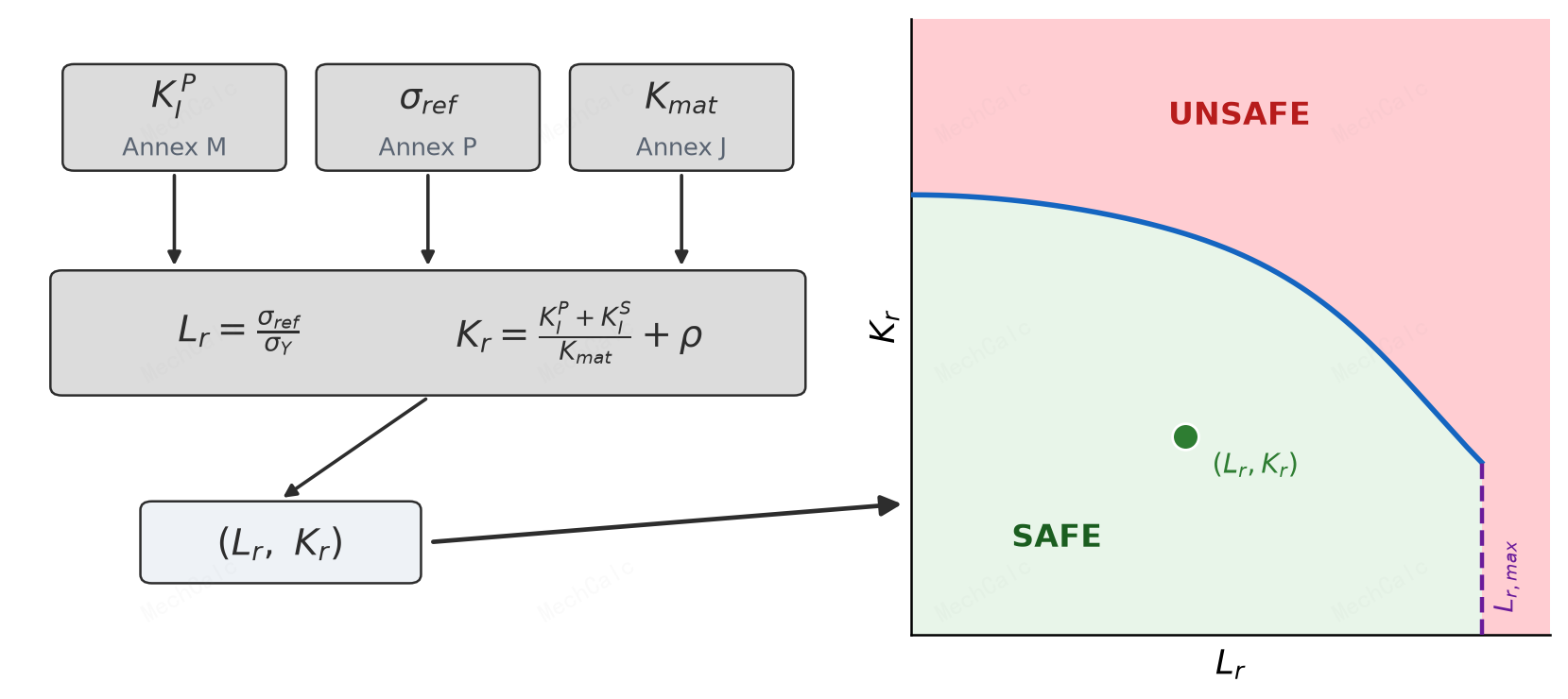
Figure 1: The BS 7910 fracture assessment at a glance. On the left is the calculation chain — three verified building blocks K_I (Annex M), σ_ref (Annex P), and K_mat (Annex J) assemble the horizontal coordinate L_r and the vertical coordinate K_r, giving an assessment point (L_r, K_r). On the right is the FAD — a point inside the failure assessment line FAL (green SAFE region) means the flaw is acceptable; on or outside the line (red UNSAFE) means it is not.
Each axis measures one failure mode, and the closer the assessment point is to the origin, the safer it is:
- Vertical axis $K_r$ (fracture ratio): how close you are to brittle fracture.
- Horizontal axis $L_r$ (load ratio): how close you are to plastic collapse.
- Failure Assessment Line (FAL) (blue): a curve $K_r = f(L_r)$ that fuses the competition between the two failures into a single boundary. A point inside the curve → the flaw is acceptable; on or outside → not acceptable.
3. The fracture-mechanics principle
Vertical axis $K_r$: how close to brittle fracture
$$K_r = \frac{K_I}{K_{mat}}$$- $K_I$ is the stress intensity factor, a measure of the strength of the singular stress field at the crack tip — it is the crack’s driving force.
- $K_{mat}$ is the material’s fracture toughness, its resistance to crack extension — the resistance.
- So $K_r$ is “driving force / resistance”. $K_r = 1$ means the driving force just equals the resistance, i.e. the point of brittle fracture. (BS 7910:2019, §7.1.1)
Horizontal axis $L_r$: how close to plastic collapse
$$L_r = \frac{\sigma_{ref}}{\sigma_Y}$$- $\sigma_{ref}$ is the reference stress, representing the “equivalent stress” level carried by the cracked section.
- $\sigma_Y$ is the material’s yield strength.
- $L_r = 1$ means the cracked section as a whole reaches yield and begins to collapse. Note that it is the cracked net section that fails first, not the entire structure yielding together — this is the difference between “net-section yielding” and “plastic collapse”. (BS 7910:2019, §7.1.1)
The FAL: fusing two failures into one line
The FAL is not a simple join of the two axes, but a curve that drops as $L_r$ rises:
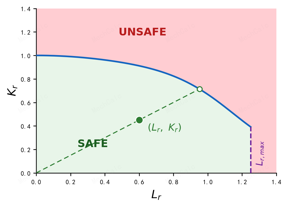
Figure 2: The FAD explained. The blue FAL falls as L_r increases; together with the axes and the vertical cut-off line L_r,max it bounds the green safe region (SAFE). The solid green dot is the assessment point (L_r, K_r); the dashed ray from the origin through the point extends to its intersection with the FAL (open dot), and the ratio between them is the load reserve factor — how much the load can still be scaled up along a proportional loading path.
Why does the curve drop? As $L_r$ rises and the crack tip enters large-scale plasticity, the plasticity blunts the tip and absorbs energy, so the material’s apparent resistance to brittle fracture actually falls; at the same time the structure moves closer to overall collapse. So at high $L_r$ the allowable $K_r$ must be pulled down. This falling curve is the balance line where the two risks — brittle fracture and plastic collapse — trade off against each other. (BS 7910:2019, §7.1.1)
Option 1 curve equation ($L_r \le 1$ branch; BS 7910:2019, §7.3, Option 1):
$$f(L_r) = \left(1 + \tfrac{1}{2}L_r^2\right)^{-1/2}\left[0.3 + 0.7\,e^{-\mu L_r^6}\right], \quad \mu = \min\!\left(0.001\,\frac{E}{\sigma_Y},\ 0.6\right)$$4. The calculation: three steps to one assessment point
Plotting the assessment point $(L_r, K_r)$ is essentially walking through the calculation chain on the left of Figure 1.
Step 1: stress intensity factor $K_I$ (Annex M)
$K_I$ describes the strength of the elastic stress field at the crack tip. Annex M of BS 7910 gives general expressions for standard geometries (plate, cylinder, sphere, …) containing flaws, with the skeleton:
$$K_I = \left(P_m M_m + P_b M_b\right) M_k\, f_w \sqrt{\frac{\pi a}{Q}}$$The physical meaning of each correction factor:
| Symbol | Name | Physical meaning |
|---|---|---|
| $M_m$ | membrane correction factor | geometric correction for the membrane-stress contribution of a surface/embedded crack (Newman–Raju polynomials) |
| $M_b$ | bending correction factor | contribution of bending stress to crack-tip $K$ |
| $M_k$ | weld-toe magnification factor | extra magnification from local stress concentration at the weld toe (= 1 with no weld) |
| $f_w$ | finite-width correction | boundary effect for a plate of finite width (≈ 1 for wide plates) |
| $Q$ | flaw shape parameter | $= 1 + 1.464\,(a/c)^{1.65}$, an elliptic-integral approximation combining the crack aspect ratio |
Before computing, the real flaw is first characterised (idealised) into a standard geometry — an enclosing regular shape stands in for the irregular measured flaw (BS 7910:2019, §7.1.2):
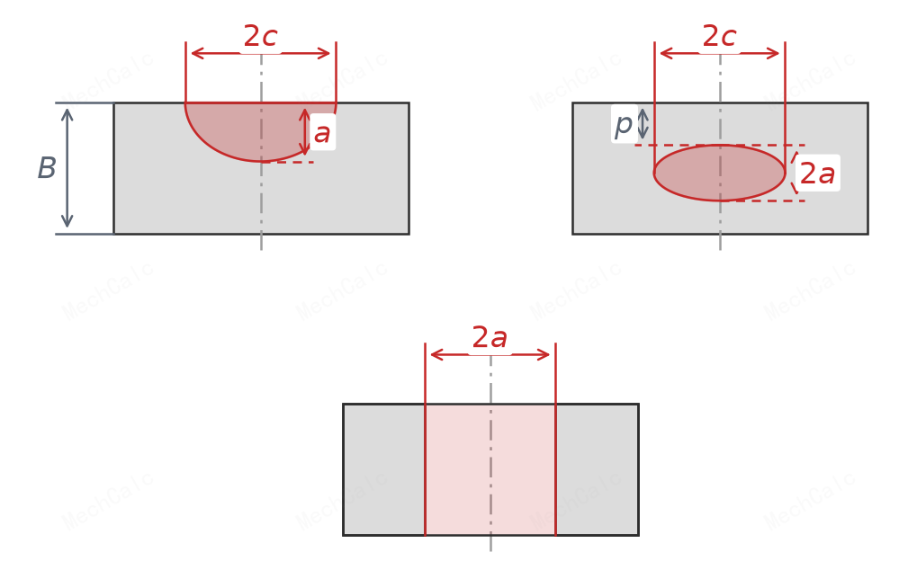
Figure 3: Size definitions for the three basic flaws. Top left, a surface crack (depth a, total length 2c, wall thickness B); top right, an embedded crack (height 2a, length 2c, distance p to the near surface); bottom, a through-thickness crack (total length 2a). Each K_I formula in Annex M corresponds to one flaw geometry.
Step 2: reference stress $\sigma_{ref}$ (Annex P)
The key idea of the reference-stress method is to map the complex plastic behaviour of a cracked structure back onto an equivalent elastic problem. This is done by defining a fictitious reference stress $\sigma_{ref}$ tied to the limit load $P_L$ of the cracked section — in essence $\sigma_{ref}$ and $P_L$ are two languages for the same thing (one in stress units, one in load units), related through the load-bearing area: $\sigma_{ref} \times A \approx P_L$.
Once $\sigma_{ref}$ is known, the horizontal coordinate is $L_r = \sigma_{ref} / \sigma_Y$. How $\sigma_{ref}$ is taken depends on the flaw type and stress distribution, and is looked up from the relevant Annex P solutions. (BS 7910:2019, Annex P)
Step 3: assembling $K_r$ and $L_r$
A real assessment usually also involves secondary stresses such as weld residual stress or thermal stress. The full assembly of the vertical coordinate is (BS 7910:2019, §7.3, Eq. 7.39):
$$K_r = \frac{K_I^P + K_I^S}{K_{mat}} + \rho$$- $K_I^P$: the SIF from primary stress (produced by external loads such as pressure or mechanical force), counted in full;
- $K_I^S$: the SIF from secondary stress (self-balancing, such as weld residual or thermal stress);
- $\rho$: the plasticity interaction correction between primary and secondary stress (BS 7910:2019, Annex R).
Why primary and secondary stresses are treated differently is the most important — and most confusing — point in Clause 7:
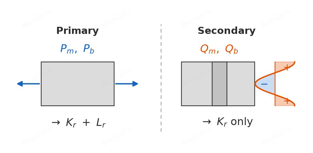
Figure 4: Primary vs secondary stress. Primary stress (Pm/Pb) is sustained by external loads and does not self-balance, so it enters both K_r and L_r. Secondary stress (Qm/Qb, e.g. weld residual stress) is self-balancing and relaxes with plastic flow, so it enters K_r only (with a plasticity-interaction correction), not L_r.
The reason: $L_r$ measures “how far from overall plastic collapse”, and overall collapse is driven by the externally sustained primary load; secondary stress is self-balancing and relaxes with plastic flow, so it cannot push the structure into collapse on its own. Therefore:
- Only primary stress enters $L_r$: $\;L_r = \sigma_{ref}/\sigma_Y$ (horizontal axis, collapse);
- Both primary and secondary stress enter $K_r$ (vertical axis, fracture), with secondary stress corrected through $\rho$.
⚠️ Key rule: when $K_I^S < 0$ (compressive, favourable secondary stress), set both $K_I^S$ and $\rho$ to zero (a conservative treatment). And $\rho$ is a separate term added outside the fraction — never put it in the denominator.
When $K_I^S = 0$ and $\rho = 0$, the expression reduces exactly to $K_r = K_I / K_{mat}$ — the basic form of the vertical axis from Section 3.
The plastic cut-off $L_{r,max}$
The FAD is cut off hard at a certain horizontal coordinate: for $L_r \ge L_{r,max}$, $f(L_r) = 0$, and the flaw is judged to fail no matter how good the toughness. The cut-off value is (BS 7910:2019, §7.3):
$$L_{r,max} = \frac{\sigma_Y + \sigma_U}{2\sigma_Y}$$The numerator $(\sigma_Y + \sigma_U)/2$ is the flow stress $\sigma_f$ (the mean of yield and tensile strength), representing the average stress level at which the material reaches full plasticity. Beyond this vertical line the structure fails by overall plastic flow, regardless of crack toughness.
FAD options: Option 1 / 2 / 3
The FAL curve has three levels of increasing accuracy (BS 7910:2019, §7.3):
| Option | Data needed | Character |
|---|---|---|
| Option 1 | only $\sigma_Y$, $\sigma_U$ | the general default, most conservative, least data-hungry (the formula in Section 3) |
| Option 2 | the material stress–strain curve | built point by point from the real hardening behaviour; usually a wider safe region |
| Option 3 | a finite-element $J$-integral solution | the most accurate, building the FAD directly from $J$; the most work |
You can start from Option 1; only when Option 1 fails and the extra margin is worth chasing do you move up a level.
5. The BS 7910 fracture assessment steps
Clause 7 lays out a complete assessment procedure (BS 7910:2019, §7.2). It can be grouped into four stages:
Stage 1 · Preparation (gather inputs)
- Define loads and stresses: identify the worst load case and split stresses into primary / secondary. (mandatory)
- Determine the fracture toughness $K_{mat}$: from tests or estimates; when data are missing, convert from Charpy energy via Annex J. (mandatory)
- Determine tensile properties: take $\sigma_Y$, $\sigma_U$, $E$ of the weakest material near the flaw. (mandatory)
- Characterise the flaw: idealise the measured flaw into a standard geometry (Figure 3), fixing $a$, $2c$, etc. (mandatory)
Stage 2 · Choose the framework
- Select and compute the FAD: choose Option 1 / 2 / 3 per §7.3, and compute the FAL curve $f(L_r)$ and the cut-off $L_{r,max}$. (mandatory)
- Choose the analysis type: an initiation analysis (single-point check) or a ductile-tearing analysis (point-locus check). (mandatory)
Stage 3 · Compute the point
- Compute $L_r$: $L_r = \sigma_{ref}/\sigma_Y$ (primary stress only). (mandatory)
- Compute $K_r$: assemble primary + secondary stress and $\rho$ per Eq. 7.39. (mandatory)
- Estimate in-service growth: if the service life includes fatigue (Clause 8), creep (Clause 9), or environmental cracking (Clause 10), compute the growth $\Delta a$ to obtain a series of assessment points that move with size. (as needed)
Stage 4 · Judge
- Plot on the FAD: a single point for initiation, a locus for tearing. (mandatory)
- Compare and judge: the position of the point/locus relative to the FAL decides PASS / FAIL. (mandatory)
- Refine if it fails: move to a higher Option, apply a constraint correction (Annex N), a weld strength-mismatch correction (Annex I), flaw re-characterisation (Annex E), and so on — each is a physically grounded argument, not a way to “game” the result. (as needed)
- Report: prepare a traceable assessment report per Annex H. (mandatory)
6. The criterion: how PASS / FAIL is judged
For the most common initiation analysis, the criterion is simply the position of the assessment point relative to the FAL (BS 7910:2019, §7.2 / §7.3):
- If $K_r \le f(L_r)$ and $L_r < L_{r,max}$ → PASS (flaw acceptable);
- If $K_r > f(L_r)$ or $L_r \ge L_{r,max}$ → FAIL (flaw not acceptable).
Telling the two failure modes apart on the diagram
- The point crosses the line in the upper-left ($L_r$ small, $K_r$ high) → brittle fracture dominates, toughness is short;
- The point crosses in the lower-right ($K_r$ small, $L_r$ approaching $L_{r,max}$) → plastic collapse dominates, capacity is short;
- Crossing near the knee of the curve → the two risks are comparable.
Reserve factors: how much margin is left
The standard itself carries no built-in safety factor, so a point sitting “just on the FAL” only means “just not failing”, with zero margin. Two reserve factors quantify the margin:
- Toughness reserve factor $F_{K_r}$: the margin from the assessment point to the FAL measured along the vertical axis;
- Load reserve factor $F_{load}$: the margin measured along the proportional-loading ray from the origin through the point (the dashed ray in Figure 2), answering “by what factor can the load still be scaled before it touches the line”.
Because there is no built-in safety factor, a sensitivity analysis is essential: perturb the flaw size, toughness, and stress each a little and check whether the point stays comfortably inside the safe region — this is the real core of engineering risk judgement.
7. A worked example (Option 1, primary stress only)
Take a surface crack in a plate under primary stress only ($K_I^S = 0$, $\rho = 0$):
| Parameter | Value | Parameter | Value | |
|---|---|---|---|---|
| membrane stress $P_m$ | 100 MPa | yield strength $\sigma_Y$ | 350 MPa | |
| bending stress $P_b$ | 50 MPa | tensile strength $\sigma_U$ | 500 MPa | |
| crack depth $a$ | 5 mm | Young’s modulus $E$ | 210 GPa | |
| crack half-length $c$ | 10 mm | fracture toughness $K_{mat}$ | 90 MPa·m$^{1/2}$ | |
| plate thickness $B$ | 25 mm | plate width $W$ | 200 mm (no weld, $M_k=1$) |
Step 1, $K_I$: $a/c = 0.5$, $a/B = 0.2$, $Q = 1 + 1.464 \times 0.5^{1.65} = 1.466$; giving $K_I \approx 15.85$ MPa·m$^{1/2}$.
Step 2, $\sigma_{ref}$: from the Annex P surface-crack solution, $\sigma_{ref} \approx 126.5$ MPa, so $L_r = 126.5/350 = 0.361$; the cut-off is $L_{r,max} = (350+500)/(2\times350) = 1.214$.
Step 3, assessment: $K_r = 15.85/90 = 0.176$; with $\mu = 0.6$, $f(0.361) \approx 0.968$.
The assessment point $(0.361,\ 0.176)$ lies well inside the curve limit $(0.361,\ 0.968)$, with a vertical margin of $0.968 - 0.176 = 0.792$.
Result: ✅ PASS, with ample reserve.
8. Common pitfalls
- “Can the crack be used” is the wrong question. What is assessed is whether the cracked structure can stay in service and whether the flaw is acceptable — not the crack itself.
- Counting secondary stress in $L_r$. Secondary stress (residual, thermal) enters $K_r$ only, never $L_r$. When unsure whether a stress is primary or secondary, treat it as primary (more conservative).
- Calling a stress “primary” just because it is large. The test is “does it drive overall plastic collapse”, not the magnitude: residual stress, even near yield in magnitude, is still treated as secondary.
- Putting $\rho$ in the denominator. $\rho$ is a separate term added outside the fraction in $K_r = \dfrac{K_I^P + K_I^S}{K_{mat}} + \rho$.
- Mixing up which tensile properties to use. A common convention: use lower-bound properties for $K_r$/$L_r$, and mean (flow-stress) properties for the FAL and $L_{r,max}$.
- Treating “on the line” as safe. The standard has no built-in safety factor, so being on the line means zero margin — a sensitivity analysis is a must.
Run it online with MechCalc
Once you understand the principle, the fastest way to learn is to try it. Use the online BS 7910 fracture assessment calculator: enter the example above (or your own flaw) and it runs Annex M ($K_I$) + Annex P ($\sigma_{ref}$) + the FAD assessment in one click, returning a PASS/FAIL verdict, reserve factors, and a live FAD chart; you can optionally include secondary stress $K_I^S$, the Annex R plasticity interaction $\rho$, an Annex J toughness estimate, and Option 2/3.
🧮 在线计算器:BS 7910 Fracture Assessment Calculator — Choose Option 1, enter the inputs from Section 7, and reproduce the PASS result L_r=0.361, K_r=0.176, f(L_r)=0.968.
The figures in this article are original MechCalc diagrams for teaching only and do not replace the BS 7910 standard. For engineering assessment, refer to the current BS 7910:2019+A1:2020.