In a BS 7910 fracture assessment, the horizontal axis $L_r$, the vertical axis $K_r$, and the failure assessment line (FAL) that separates “safe” from “unsafe” — how the assessment point is computed and how the verdict is read — are covered thoroughly in the BS 7910 Fracture Assessment — A Concise Guide . This article covers one thing only: Clause 7 gives three ways to draw that FAL curve (Option 1 / 2 / 3). They step up in the material data they need, in computational accuracy and in conservatism; understanding their differences is a key step to doing a fracture assessment “correctly and economically”.
1. One FAD, three ways to draw it
First, an easily-missed fact: the three options change only how the failure assessment line $f(L_r)$ is drawn; the assessment point $(L_r,\,K_r)$ is computed identically in all three.
That is, whichever option you choose:
- the horizontal load ratio $L_r = \dfrac{P}{P_L(a,\sigma_Y)} = \dfrac{\sigma_{ref}}{\sigma_Y}$ is still computed from the primary load only (BS 7910:2019, §7.3.7, Eq. (7.40));
- the vertical fracture ratio $K_r$ still assembles the primary stress $K_I^{\,p}$, the secondary stress $K_I^{\,s}$ and the plasticity interaction correction as below (BS 7910:2019, §7.3.6, Eq. (7.39)):
The only difference between the three options is what that FAL curve $f(L_r)$ looks like. In other words, choosing an option means choosing “how much material data to trace the boundary with” — the more data, the closer the boundary follows the material’s real behaviour.
Before comparing them, one hard boundary shared by all three must be set up first.
The plastic-collapse cut-off $L_{r,\max}$: the right wall for all three curves
Whichever option, the horizontal axis has an upper limit $L_{r,\max}$. Once $L_r$ reaches it, the structure fails by overall plastic flow of the flawed section no matter how high the toughness, and $f(L_r)$ is taken as zero (BS 7910:2019, §7.3.2, Eq. (7.25)):
$$L_{r,\max} = \frac{\sigma_Y + \sigma_U}{2\sigma_Y}$$The numerator $(\sigma_Y+\sigma_U)/2$ is the flow stress $\sigma_f$ (the mean of yield and tensile strength), representing the average stress level as the material goes fully plastic. So $L_{r,\max}$ is essentially “the flow stress relative to the yield strength”, computed with mean (not lower-bound) tensile properties. This vertical wall applies to all three options alike.
2. Option 1: yield and tensile strength only
Option 1 is the option with the lowest data need and the most common in practice: it does not need a full stress-strain curve — the whole FAL can be set from the yield strength $\sigma_Y$, tensile strength $\sigma_U$ and elastic modulus $E$ alone (BS 7910:2019, §7.3.3). It is a general approximate lower bound the standard fitted from data on many common structural steels.
Continuous-yielding materials (no yield plateau)
$$f(L_r) = \left(1 + \tfrac{1}{2}L_r^2\right)^{-0.5}\left[\,0.3 + 0.7\exp\!\left(-\mu L_r^6\right)\right] \quad (L_r \le 1)$$$$f(L_r) = f(L_r{=}1)\;L_r^{\,(N-1)/(2N)} \quad (1 < L_r < L_{r,\max})$$The two material parameters are (BS 7910:2019, §7.3.3, Eq. (7.26), (7.27)):
$$\mu = \min\!\left(0.001\frac{E}{\sigma_Y},\; 0.6\right), \qquad N = 0.3\left(1 - \frac{\sigma_Y}{\sigma_U}\right)$$Reading: the $(1+\tfrac{1}{2}L_r^2)^{-0.5}$ outside the bracket comes from a small-scale-yielding correction, and the exponential decay inside the bracket captures the rapid rise of driving force as yield is approached; the lower the yield-to-tensile ratio $\sigma_Y/\sigma_U$ (the stronger the strain hardening), the larger $N$, and the more gently the curve drops in the $L_r>1$ branch.
Discontinuous-yielding materials (with a yield plateau)
Many low-carbon and C-Mn steels have a yield plateau (Lüders plateau) at the lower yield strength — the stress barely rises while the strain suddenly grows. The FAL for these materials switches to another set of equations, with a vertical drop at $L_r = 1$ (BS 7910:2019, §7.3.3, Eq. (7.29)–(7.33)):
$$\lambda = 1 + \frac{E\,\Delta\varepsilon}{R_{eL}}$$Why the vertical drop? At $L_r=1$ (the reference stress just reaches yield) the material runs a strain increment $\Delta\varepsilon$ along the yield plateau at nearly constant stress; the plastic deformation capacity of the flawed section is released abruptly, so the allowed $K_r$ drops like a cliff from its pre-plateau value to a lower post-plateau value. The parameter $\lambda$ measures the “total strain at the end of the yield plateau” relative to the “initial elastic yield strain” — the longer the plateau (the larger $\Delta\varepsilon$), the larger $\lambda$ and the deeper the drop.
Do not use the wrong yielding type: for a steel with a yield plateau, using the continuous-yielding equation (7.26) overestimates the safety margin near $L_r \approx 1$ — an unsafe error. For deciding whether a material has a yield plateau, see §7.1.3.6. (See also the dedicated article, Continuous or Discontinuous Yielding? )
3. Option 2: the true stress-true strain curve, the general option
Option 2 builds the FAL from the mean uniaxial true stress-true strain curve at the assessment temperature; it is suitable for all metals regardless of stress-strain behaviour, so it is more general than Option 1 and its FAL follows the material more closely (BS 7910:2019, §7.3.4, Eq. (7.34)):
$$f(L_r) = \left(\frac{E\,\varepsilon_{ref}}{L_r\,\sigma_Y} + \frac{L_r^3\,\sigma_Y}{2\,E\,\varepsilon_{ref}}\right)^{-0.5} \quad (L_r < L_{r,\max})$$Here $\varepsilon_{ref}$ is the true strain at the true stress $\sigma_{ref} = L_r\sigma_Y$. A handy reading: the denominator $L_r\sigma_Y$ of the first term is exactly the reference stress $\sigma_{ref}$, so the first term $E\varepsilon_{ref}/\sigma_{ref}$ is the inverse of “the elastic-strain estimate $\sigma_{ref}/E$ over the true reference strain $\varepsilon_{ref}$”. As $L_r$ rises and the material goes plastic, $\varepsilon_{ref}$ departs from the elastic value, the first term grows, and $f(L_r)$ falls — this is how the material’s real plastic deformation capacity is written into the FAL.
To use Option 2, you must first build the true stress-true strain curve from tensile data (or a Ramberg-Osgood fit, Eq. (7.4)–(7.7)), especially the knee below 1% strain — the FAD shape near the knee at $L_r\approx1$ depends heavily on the quality of that data. The full step-by-step procedure for building the FAL point by point is a separate topic.
True stress ≠ engineering stress: Option 2 requires true stress-true strain input. A tensile test gives engineering stress-engineering strain directly; feeding it in without converting to true values in the plastic range causes a clear error.
4. Option 3: directly from elastic-plastic $J$ — the most accurate but not general
Option 3 targets a specific material, geometry and loading type: for the flawed structure it runs both an elastic analysis and an elastic-plastic analysis (usually by finite element), and defines the FAL from the ratio of their $J$-integrals (BS 7910:2019, §7.3.5, Eq. (7.36)):
$$f(L_r) = \sqrt{\frac{J_e}{J}} \quad (L_r < L_{r,\max})$$where $J_e$ is the $J$ from an elastic analysis at a given $L_r$ load and $J$ is the $J$ from an elastic-plastic analysis at the same load. Reading: the ratio $J_e/J$ measures “how much a purely elastic calculation would underestimate the true driving force” — the more plasticity, the more $J \gg J_e$, the smaller $\sqrt{J_e/J}$, and the lower the FAL.
Option 3 is the most accurate but also the most costly: it is not general — one curve is valid only for the specific configuration it was derived for — so it is used only in specific critical assessments as an alternative to Options 1 and 2.
5. Comparing the three: how data, accuracy and conservatism step up
Put the three FALs on one failure assessment diagram and the pattern is clear at a glance: “more data → curve further out → larger acceptable region”:
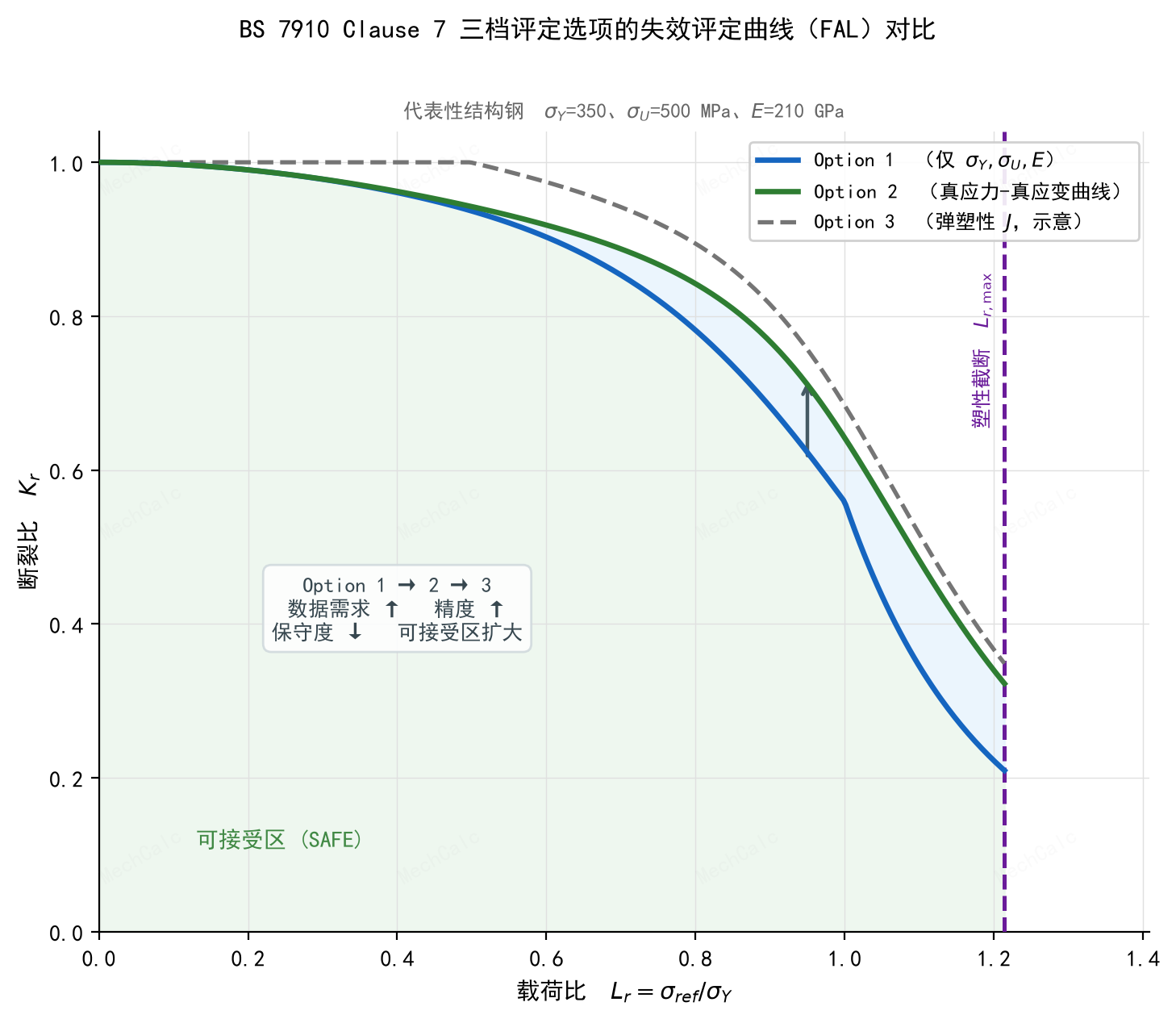
Figure 1: The three Clause 7 assessment options’ failure assessment lines compared (representative structural steel σ_Y=350, σ_U=500 MPa, E=210 GPa). Option 1 (blue, needs only σ_Y/σ_U/E) and Option 2 (green, from the true stress-true strain curve) are computed exactly from the code equations; Option 3 (grey dashed, elastic-plastic J) is schematic — it must be found by finite element J for a specific configuration and is not a general curve. All three share the same plastic-collapse cut-off L_r,max at the right. The higher the data need, the closer the FAL follows the material’s real behaviour, the less conservative the margin, and the larger the acceptable flaw.
The trade-off in one line:
| Option | Data needed | Cost | Character |
|---|---|---|---|
| Option 1 | Only $\sigma_Y$, $\sigma_U$, $E$ | Lowest (plug into the general formula) | General approximate lower bound, least data, the engineering default starting point |
| Option 2 | True stress-true strain curve (especially the <1% knee) | Medium (built point by point) | Suitable for all metals, follows the material’s real hardening behaviour |
| Option 3 | Elastic-plastic $J$-integral solution (usually FEA) | Highest (numerical analysis) | Most accurate, valid only for a specific configuration, not general |
In general, conservatism runs Option 1 > Option 2 > Option 3 — the further along, the closer to reality and the less margin spent.
An exception you must know: low-strain-hardening materials
“Higher option = less conservative” is not absolute. For some low-strain-hardening (very weak work-hardening) materials, the Option 2 curve can actually fall inside the general Option 1 curve (BS 7910:2019, §7.4.2).
The reason: Option 1 is an approximate lower bound the standard fitted from common structural steels. If a material’s stress-strain curve flattens quickly after yield, then just past yield its plastic deformation (and elastic-plastic $J$) grows far faster than for ordinary materials, so $f(L_r)$ drops sharply and falls inside the Option 1 curve. Here Option 1 is on the unsafe side, and Option 2, based on the real stress-strain curve, must be used to envelop the risk faithfully. So moving up an option is not only about “spending less margin” — sometimes it is about “correcting the distortion of the general curve for a specific material”.
How to choose: by scenario and data completeness
Which option to choose depends on the completeness of the data at hand and the urgency of the assessment:
- Routine quick assessment, limited material data: start from Option 1. It needs the least data and is the safest; in most cases, if it passes there is no need to go further.
- Option 1 fails but the margin is worth pursuing, and you have (or can afford) the material’s true stress-strain curve: move up to Option 2 and use the real hardening behaviour to recover the margin Option 1 “buried”.
- Margin is critical, the configuration is important, and numerical analysis is justified: use Option 3, run an elastic-plastic $J$ analysis for the specific configuration, and make the assessment as realistic as possible.
- For a low-strain-hardening material: even if Option 1 passes, check with Option 2 — because Option 1 may be non-conservative here (see above).
6. Three common pitfalls
- Pitfall 1: using the wrong yielding type. For a carbon steel with a yield plateau, not using the discontinuous-yielding equations with their drop segment badly overestimates the load-bearing safety margin in the $L_r\ge1$ region (§7.4.2).
- Pitfall 2: treating “higher option” as “safer”. Moving up an option only means the calculation follows reality more closely and removes some conservative assumptions of the lower option (saving margin) — it adds no extra safety. The BS 7910 method has no built-in safety factor of its own — the assessment point lying inside the curve only means “in theory it just does not fail”. The real safety margin must be confirmed by the user with a sensitivity analysis on the flaw size, stress, toughness and other inputs (§7.1.12).
- Pitfall 3: putting $\rho$ inside the fraction. The plasticity interaction correction $\rho$ is a separate term added outside the fraction, $K_r = \dfrac{K_I^{\,p}+K_I^{\,s}}{K_{mat}} + \rho$ — never inside the numerator bracket or the denominator. The standard also gives an equivalent multiplier form $K_r = \dfrac{K_I^{\,p}+V\,K_I^{\,s}}{K_{mat}}$ (Eq. (7.38)), but once you use the additive term $\rho$ it must be fully separate (BS 7910:2019, §7.3.6).
Note: all three FALs can be used for ductile-tearing analysis (§7.3.8) — assume a set of tearing amounts, compute a string of assessment points with the corresponding enhanced toughness, and join them into a locus; where the locus is tangent to the chosen FAL is the instability point. Changing the option only changes the curve being compared against; the tearing analysis procedure is unchanged.
Try the three options online with MechCalc
Once the differences are clear, hands-on is quickest. In the online BS 7910 fracture assessment calculator, the FAD Option drop-down switches between Option 1 / 2 / 3: Option 1 needs only yield/tensile strength, Option 2 provides Ramberg-Osgood parameters, and Option 3 lets you enter the elastic $J_e$ and elastic-plastic $J$ from your own analysis. Switch options and watch in real time how the FAL curve and assessment point move, and how the reserve factors tighten or loosen.
🧮 在线计算器:BS 7910 Fracture Assessment Calculator — Switch between Option 1 / 2 / 3 in the 'FAD Option' drop-down and compare in real time the margin at the same assessment point under the three FALs.
The figures here are original MechCalc illustrations for teaching only; they do not replace the BS 7910 text. The Option 3 curve in the figure is schematic; in practice it must be determined by finite element J for a specific configuration. For engineering assessment use the current BS 7910:2019+A1:2020.