A fracture assessment watches two things at once — how close to brittle fracture, and how close to plastic collapse. Annex M (the stress intensity factor) covers the first and gives the vertical axis $K_r$ of the Failure Assessment Diagram (FAD); this guide’s reference stress $\sigma_{ref}$ (Annex P) covers the second and gives the horizontal axis $L_r$. Together they complete the Clause 7 fracture assessment .
Prologue: the horizontal axis measures “how close to plastic collapse”
A cracked structure can fail along two paths: brittle fracture, where the crack-tip driving force exceeds the toughness, and plastic collapse, where the cracked section as a whole yields and loses its capacity. The first is measured by $K_I$ (vertical axis); the second relies on the reference stress $\sigma_{ref}$ (horizontal axis).
1. What the reference stress is
The reference stress $\sigma_{ref}$ is an equivalent uniform stress obtained by normalising the complex geometry and loading of a cracked structure. To be clear from the start:
- It is not the real stress at the crack tip (that is what $K_I$ describes);
- It is a yardstick for “how close to plastic collapse”: when $\sigma_{ref}$ reaches the material yield strength $\sigma_Y$, the remaining load-bearing section around the flaw (the ligament) yields as a whole — the onset of plastic collapse. (BS 7910:2019, §P.2)
2. The core idea of the reference-stress method
A real cracked structure is an elastic-plastic problem, and computing it exactly means a complex $J$-integral (non-linear finite elements). The reference-stress method (Ainsworth, 1984) bypasses this:
Use the material’s uniaxial tensile (yield) properties and the structure’s plastic limit load to estimate the elastic-plastic behaviour of the cracked structure by equivalence.
Concretely, a closed-form formula gives the structure’s plastic limit load $P_L$ (or the equivalent $\sigma_{ref}$) directly, which then drives the plasticity correction — saving the precise non-linear analysis.
$\sigma_{ref}$ and the limit load $P_L$ are really two languages for the same thing (stress language vs load language), linked by the load-bearing area:
$$L_r = \frac{P}{P_L} = \frac{\sigma_{ref}}{\sigma_Y}$$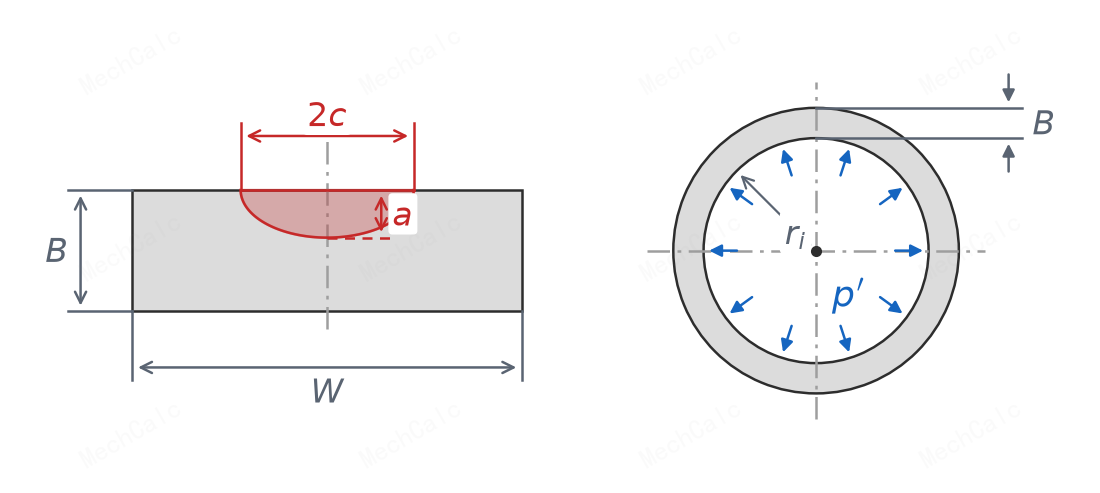
Figure 1: Plate/shell geometry and the load-bearing section. The reference-stress method treats ‘a cracked section under complex loading’ as ‘a uniform stress σ_ref acting on the load-bearing section’ — σ_ref reaching the yield strength corresponds to the plastic limit load P_L of the cracked section.
3. How $\sigma_{ref}$ gives the horizontal axis $L_r$
Once $\sigma_{ref}$ is known, the FAD horizontal axis is the load ratio:
$$L_r = \frac{\sigma_{ref}}{\sigma_Y}$$- $L_r < 1$: the load is well short of plastic collapse, the ligament essentially elastic;
- $L_r = 1$: the cracked section just reaches yield (near the “knee” of the FAL);
- $L_r \ge L_{r,max}$: whether or not it fractures, the structure has failed by overall plastic flow. (BS 7910:2019, §7.3.2)
Note: only primary stress enters $L_r$. Secondary stress (residual, thermal) is self-balancing and relaxes with plasticity; it does not drive overall collapse, so it stays out of the horizontal axis and enters only the vertical axis $K_r$.
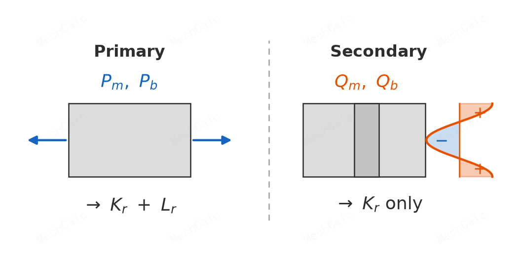
Figure 2: Primary vs secondary stress. Primary stress (Pm/Pb) is sustained by external loads and enters both K_r and L_r; secondary stress (Qm/Qb) is self-balancing and enters K_r only, not L_r. σ_ref and L_r are computed from primary stress alone.
4. The general Annex P framework
Most Annex P solutions (plate and shell types) write $\sigma_{ref}$ as a combination of membrane stress $P_m$ and bending stress $P_b$. The signature form is for a through-thickness crack in a plate (BS 7910:2019, §P.4):
$$\sigma_{ref} = \frac{P_b + \sqrt{P_b^2 + 9P_m^2\,(1-\alpha)^2}}{3\,(1-\alpha)^2}$$Many other geometry solutions are variations of it. Here $\alpha$ (written $a''$ in some solutions) is the equivalent flaw parameter, representing how much the flaw weakens the load-bearing section:
- $\alpha=0$: no flaw, $\sigma_{ref}=\sigma_Y$ (the denominator $(1-\alpha)^2=1$; for pure membrane it reduces to $\sigma_{ref}=P_m$);
- larger $\alpha$: less ligament, more capacity lost, the denominator $(1-\alpha)^2$ shrinks fast and $\sigma_{ref}$ rises sharply.
Physically, the denominator $(1-\alpha)^2$ is exactly the non-linear degradation of net-section capacity: the deeper the crack, the higher the equivalent stress the remaining ligament needs to carry the same load.
Constraint and boundary conditions also affect $\sigma_{ref}$: fixed-grip (restrained) vs pin-jointed (free rotation), plane stress vs plane strain — each gives a different solution; in general, more constraint means a higher limit load and a lower $\sigma_{ref}$. (BS 7910:2019, §P.5)
5. The plastic cut-off $L_{r,max}$ and the flow stress
The FAD horizontal axis has a hard cut-off line: for $L_r \ge L_{r,max}$ the flaw is judged to fail by plastic collapse, regardless of toughness (BS 7910:2019, §7.3.2):
$$L_{r,max} = \frac{\sigma_Y + \sigma_U}{2\sigma_Y}$$The numerator $(\sigma_Y+\sigma_U)/2$ is the flow stress $\sigma_f$ — the average stress level between general yield and tensile failure. Limit-load analysis treats the material as “elastic-perfectly-plastic”, taking the flow stress once plastic. $L_{r,max}$ is the ratio of flow stress to yield strength, usually between 1.1 and 1.4 (not 1).
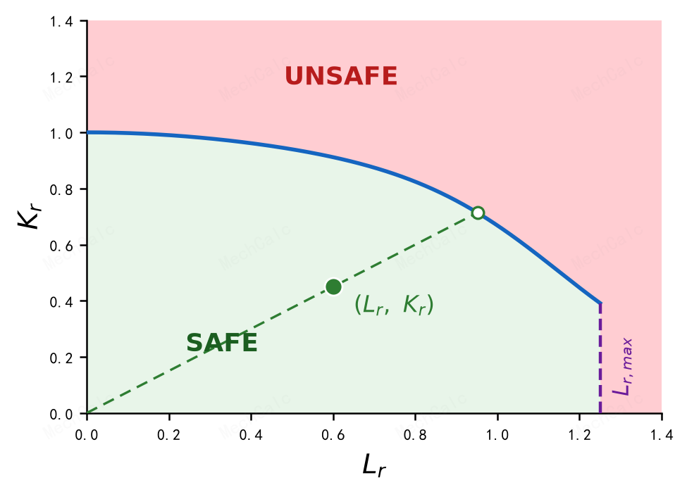
Figure 3: The Failure Assessment Diagram (FAD). The horizontal axis L_r comes from σ_ref/σ_Y; the vertical dashed line L_r,max on the right is the plastic cut-off — the further right the assessment point, the closer to plastic collapse, and beyond L_r,max it fails. Inside the green safe region and below the curve is acceptable.
6. Solutions for different geometries: local vs global collapse
Annex P §P.4–P.14 give reference-stress / limit-load solutions by geometry family (plate through/surface/embedded/corner, cylinder axial/circumferential, sphere, round bar/bolt, welded mismatch, etc.), covering pressurised thick-wall cylinders and the Folias bulging of axial cracks in a cylinder. The method is “match to the right entry”: fix the flaw geometry → find the section → check the load type and applicable range → apply the formula.
One key distinction: local collapse vs global (net-section) collapse:
- Local collapse: the remaining ligament $(B-a)$ at the flaw yields first; the local solution gives a higher $\sigma_{ref}$ (more conservative).
- Global collapse: the mean stress over the whole cracked section reaches yield; the global solution is closer to reality.
For surface / embedded flaws both solutions are given; which mode arrives first is judged from the plate width $W$ versus the flaw characteristic size $2(c+B)$: a wide plate with a small flaw tends local, a large flaw or a narrow plate tends global. A through-thickness flaw has no remaining ligament and is always global collapse. (BS 7910:2019, §P.3 / §P.5)
7. Calculation steps
From “geometry + load + crack size + material strength” to “computed $\sigma_{ref}$, $L_r$, $L_{r,max}$” (BS 7910:2019, §P and §7.2):
- Prepare inputs: geometry ($W$, $B$, cylinder diameters), flaw ($a$, $c$, position), primary loads (tension / moment / pressure), material strengths $\sigma_Y$, $\sigma_U$. (mandatory)
- Judge the collapse mode: use the plate-width rule to decide local or global collapse, which fixes the solution to use. (mandatory)
- Select the Annex P solution: match the flaw geometry / position / load to the right §P.4–P.14 entry. (mandatory)
- Convert to membrane / bending stress: turn the actual loads into $P_m=F/(WB)$, $P_b=6M^b/(WB^2)$, etc. (as needed)
- Compute $\sigma_{ref}$: substitute $P_m$, $P_b$ and the flaw parameter $\alpha$. (mandatory)
- Compute the load ratio $L_r=\sigma_{ref}/\sigma_Y$. (mandatory)
- Compute the plastic cut-off $L_{r,max}=(\sigma_Y+\sigma_U)/(2\sigma_Y)$; if $L_r\ge L_{r,max}$ it is unacceptable outright. (mandatory)
- Into the FAD: plot the assessment point with the horizontal coordinate $L_r$ and the vertical coordinate $K_r$ from Annex M , and judge. (mandatory)
8. Common pitfalls
- Treating $\sigma_{ref}$ as the crack-tip stress: $\sigma_{ref}$ is the equivalent uniform stress over the cracked section and measures plastic collapse; the real crack-tip stress is described by $K_I$. They belong to the horizontal and vertical axes respectively.
- Thinking a larger $\sigma_{ref}$ is safer: the opposite — a larger $\sigma_{ref}$ means a larger $L_r$, hence closer to collapse and less safe. The local solution gives a larger, more conservative $\sigma_{ref}$.
- Counting secondary stress in $L_r$: only primary stress enters $L_r$; residual / thermal stress enters $K_r$ only.
- Thinking $L_{r,max}=1$: $L_{r,max}=(\sigma_Y+\sigma_U)/(2\sigma_Y)>1$ (about 1.1–1.4); $L_r=1$ is only the knee, not the cut-off.
- Ignoring local vs global: for surface / embedded flaws both solutions must be checked, taking whichever mode arrives first by the plate-width rule; choosing wrong is non-conservative.
Compute $\sigma_{ref}$ online with MechCalc
Once you understand the principle, the fastest way to learn is to try it. Use the online BS 7910 Annex P calculator: choose the flaw geometry and solution, enter the crack size and primary stresses, and it computes $\sigma_{ref}$, $L_r$ and the plastic cut-off $L_{r,max}$ per Annex P, with a white-box derivation; it covers 33 geometries (plates, thin/thick cylinders, spheres, round bars/bolts).
🧮 在线计算器:BS 7910 Annex P — Reference Stress Calculator — Choose the geometry solution, enter a/c/B/W and Pm/Pb, and get σ_ref, L_r and L_r,max.
The figures in this article are original MechCalc diagrams for teaching only and do not replace the BS 7910 standard. For engineering assessment, refer to the current BS 7910:2019+A1:2020.