The first step of a fracture assessment is to compute the stress intensity factor $K_I$ at the crack tip. This guide explains what $K_I$ is and how BS 7910 Annex M computes it — from the general master formula and its correction factors to the common semi-elliptical surface-crack solution and the weld-toe correction. It feeds the vertical axis $K_r$ of the Failure Assessment Diagram (FAD), and together with Annex P (reference stress) for the horizontal axis $L_r$ completes the Clause 7 fracture assessment .
Prologue: at the crack tip, the stress is “infinite”
The first question in a fracture assessment is: how strong is this crack’s driving force?
Ordinary strength design uses “working stress < allowable stress”. But once a crack is present, linear-elastic theory says the stress at the crack tip goes to infinity — there is no finite stress value left to compare with an allowable stress. Fracture mechanics uses a new measuring stick: the stress intensity factor $K_I$.
1. Why $K_I$, and not ordinary stress
The stress field near a crack tip has a general form (linear-elastic fracture mechanics):
$$\sigma_{ij} = \frac{K_I}{\sqrt{2\pi r}}\, f_{ij}(\theta) + \cdots$$where $r$ is the distance to the tip and $\theta$ is the angle. As $r \to 0$ the stress diverges like $1/\sqrt{r}$ — this is the crack-tip stress singularity.
The key point: although the tip stress is infinite, the strength of the whole singular field is set by a single coefficient, and that coefficient is $K_I$. So:
- Ordinary stress is infinite at the tip and cannot be used directly; $K_I$ is a finite, computable, measurable quantity.
- Once $K_I$ is known, the stress/strain/displacement field near the tip is fully determined (same shape, only the magnitude differs).
- Different geometries, crack sizes, and loads can all be measured with the same $K_I$.
$K_I$ has units of $\mathrm{MPa}\sqrt{\mathrm m}$. Do not confuse it with the dimensionless stress concentration factor $k_t$, which describes stress magnification at a smooth geometric feature with no crack — a different thing entirely.
2. $K_I$ and fracture toughness: the brittle-fracture criterion
$K_I$ is the crack’s driving force; the material’s resistance to crack extension is its fracture toughness $K_{mat}$ (measured by test, varying with temperature/constraint/thickness). Comparing the two gives the brittle-fracture criterion:
$$K_I \ge K_{mat} \quad\Rightarrow\quad \text{unstable crack extension (brittle fracture)}$$In the FAD, the vertical axis is exactly the fracture ratio $K_r = K_I/K_{mat}$, measuring “how close to brittle fracture”. So the $K_I$ computed by Annex M is the raw material fed to the FAD’s vertical axis.
3. The general Annex M framework
Annex M fits every geometry’s $K_I$ solution into one master formula (BS 7910:2019, §M.1, Eq. M.1):
$$K_I = (Y\sigma)\sqrt{\pi a}$$Three ingredients: $\sqrt{\pi a}$ is the square-root term of the characteristic crack size $a$; $\sigma$ is the driving stress; $Y$ is the collective name for the geometric correction factors that carry an “ideal infinite plate” over to a “real finite component”. All of Annex M’s work is writing the specific $Y\sigma$ for each geometry.
For primary stress, $Y\sigma$ expands as (BS 7910:2019, §M.1, Eq. M.4):
$$(Y\sigma)_p = M f_w\left[k_{tm}M_{km}M_m\,P_m + k_{tb}M_{kb}M_b\big(P_b+(k_m-1)P_m\big)\right]$$It looks fierce, but it is simply a membrane-stress term plus a bending-stress term, each magnified by a string of correction factors. Secondary stress is far simpler (BS 7910:2019, §M.1, Eq. M.5): $(Y\sigma)_s = M_m Q_m + M_b Q_b$.
The physical meaning of each correction factor:
| Symbol | Name | Physical meaning | When = 1 |
|---|---|---|---|
| $M_m$ / $M_b$ | membrane / bending magnification factor | geometric magnification of $K_I$ by crack shape and position | given by each geometry solution |
| $M$ | bulging factor | extra magnification from the shell wall bulging out at the crack under internal pressure | flat plate / no bulging |
| $f_w$ | finite-width correction | net-section reduction and stress concentration when the crack takes up much of the section | crack relatively small |
| $M_{km}$ / $M_{kb}$ | weld-toe magnification factor | extra magnification when the crack sits in the local stress concentration at a weld toe | not at a weld toe |
| $k_{tm}$ / $k_{tb}$ | structural stress concentration factor | stress concentration at a gross structural discontinuity (nozzle, joint) | no structural discontinuity |
| $k_m$ | misalignment factor | axial misalignment / angular distortion turns membrane stress into extra bending $(k_m-1)P_m$ | no misalignment |
Here $P_m$, $P_b$ are primary stresses (from external loads: pressure, tension, moment) and $Q_m$, $Q_b$ are secondary stresses (self-balancing: weld residual stress, thermal stress). The two play different roles in the FAD:
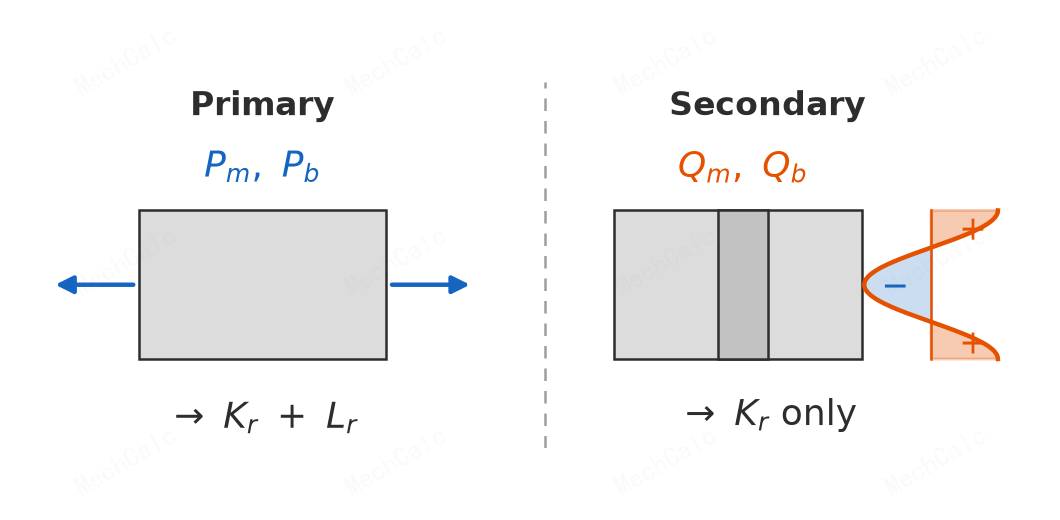
Figure 1: Primary vs secondary stress. Primary stress (Pm/Pb) is sustained by external loads and does not self-balance, so it enters both K_r and L_r. Secondary stress (Qm/Qb, e.g. weld residual stress) is self-balancing and relaxes with plastic flow, so it enters K_r only (with a plasticity-interaction correction), not L_r.
Primary $K_I^P$ and secondary $K_I^S$ add into the vertical axis: $K_r=(K_I^P+K_I^S)/K_{mat}+\rho$. When $K_I^S<0$ (compressive, favourable secondary stress), set both $K_I^S$ and $\rho$ to zero (a conservative treatment).
4. The most common solution: the semi-elliptical surface crack
In practice most surface flaws (weld-toe cracks, fatigue cracks, corrosion pits) are characterised as semi-elliptical surface cracks and use the Newman–Raju solution (BS 7910:2019, §M.4.1) — the workhorse of Annex M.
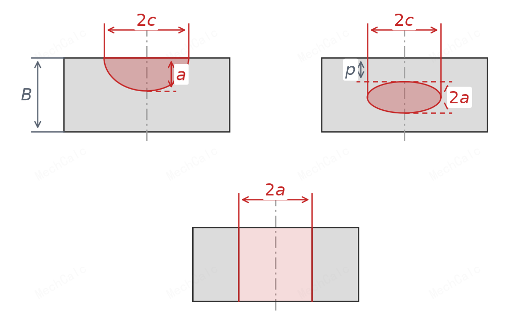
Figure 2: Size definitions for the three basic flaws. Top left, a surface crack (depth a, total length 2c, wall thickness B); top right, an embedded crack (height 2a, length 2c, distance p to the near surface); bottom, a through-thickness crack (total length 2a). A semi-elliptical surface crack is described by depth a and half-length c; the aspect ratio a/c fixes how round or flat it is.
The membrane magnification factor under tension (BS 7910:2019, §M.4.1, Eq. M.10):
$$M_m = \left[M_1 + M_2\left(\tfrac{a}{B}\right)^2 + M_3\left(\tfrac{a}{B}\right)^4\right]\frac{g\,f_\theta}{\Phi}$$The bracket is a polynomial in crack depth $a/B$ (the coefficients $M_1,M_2,M_3$ depend only on the aspect ratio $a/c$, with separate sets for $a/2c\le 0.5$ and $>0.5$); $\Phi$ is the elliptic shape factor $\Phi=\big[1+1.464(a/c)^{1.65}\big]^{0.5}$; $g$ and $f_\theta$ describe the variation along the elliptical front. Bending does not start from scratch: it takes $M_b=H\cdot M_m$ (BS 7910:2019, §M.4.1, Eq. M.12), where $H$ folds in the through-thickness decay of bending stress.
Evaluation points: deepest point A and surface point C
$K_I$ varies along the semi-elliptical front, so two special points are evaluated:
- Deepest point A ($\theta=\pi/2$): the deepest part of the crack, deciding “will it break through the wall”.
- Surface point C ($\theta=0$): where the crack meets the free surface, deciding “will it grow longer along the surface”.
Both points must be evaluated for a surface crack (BS 7910:2019, §7.2.12); take the more critical one into the FAD. Which point becomes critical first depends on the aspect ratio and the load type (tension / bending).
The finite-width correction for a surface crack is $f_w=\big\{\sec\big[(\pi c/W)(a/B)^{0.5}\big]\big\}^{0.5}$: the smaller the crack relative to the plate width, the closer $f_w\to 1$; the longer and deeper it is, the larger $f_w$. The applicable limit is roughly $2c/W\le 0.8$.
5. Welded joints: the weld-toe magnification factor $M_k$
If the crack sits at a weld toe (where the weld meets the parent material), there is a strong local stress concentration and $K_I$ must be multiplied by an extra weld-toe magnification factor $M_k$ (BS 7910:2019, §M.11). $M_k$ starts high at the surface and decays quickly with depth, returning to 1 at about 30% of the wall thickness:
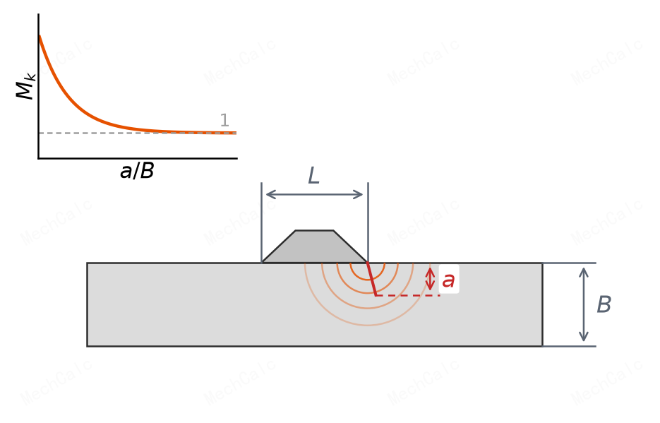
Figure 3: The weld-toe magnification factor Mk versus crack depth. For a very shallow crack (near the weld-toe surface concentration) Mk is clearly above 1; as the crack deepens out of the local weld-toe field, Mk falls quickly to 1 (the parent-material field). Membrane and bending each have their own Mkm/Mkb curve.
Use $M_k$ only when the crack is at a weld toe; otherwise take 1. Likewise: $f_w$ is used only when the crack takes up a large part of the section, $k_m$ only when there is misalignment, and the bulging factor $M$ only for axial cracks in a pressurised shell — adding corrections at will ruins the result.
6. Solutions for different geometries (overview)
Annex M gives solutions by geometry family; choosing a solution is “matching to the right entry” (BS 7910:2019, Annex M):
| Geometry | Crack types covered | Key feature |
|---|---|---|
| Flat plate | through / edge / semi-elliptical surface / embedded / corner | $M_m/M_b$ polynomials + $f_w$ |
| Cylinder, axial | through / internal & external surface / embedded | bulging factor $M$ under internal pressure |
| Cylinder, circumferential | through / internal surface | global moment converted to equivalent membrane stress |
| Sphere | equatorial through | bulging + influence coefficients |
| Round bar / bolt | surface / circumferential | round section + thread geometry |
| Welded joint | weld toe / weld root | weld-toe magnification factor $M_k$ |
Four questions to pick a solution: curved shell or flat plate (bulging or not)? surface or through (two points to evaluate or not)? finite-length or extended (3-D semi-ellipse vs 2-D)? at a weld toe (need $M_k$ or not)?
⚠️ Two rules: (1) no extrapolation — every solution has an applicable range of $a/B$, $a/c$, $2c/W$; going outside it distorts the result badly, so use the weight-function polynomial solution or finite elements instead; (2) do not count bulging twice — either “flat-plate solution times $M$” or “a cylinder solution that already includes bulging”, never both.
7. Calculation steps
From “geometry + load + crack size” to “computed $K_I$” (BS 7910:2019, §M and §7.2):
- Characterise the flaw: idealise the measured flaw into a standard shape (surface / embedded / through / corner) and measure $a$, $c$, $B$, $W$. (mandatory)
- Resolve the stress: split it into membrane $P_m$ + bending $P_b$ (fit a polynomial for a non-linear profile); separate primary $P$ from secondary $Q$. (mandatory)
- Select the geometry solution: match the flaw geometry to the right Annex M entry and check its applicable range. (mandatory)
- Compute the correction factors: as needed, $M_m/M_b$, $f_w$ (only if the crack exceeds ~10% of the section), $M_k$ (weld toe), $M$ (pressurised shell), $k_m$ (misalignment). (as needed)
- Assemble $K_I$: multiply term by term per Eq. M.4 for $K_I^P$, and per Eq. M.5 for $K_I^S$. (mandatory)
- Evaluate at the right point: for a surface crack compute the deepest point A and the surface point C, taking the more critical. (mandatory)
- Into the FAD: use $K_r=(K_I^P+K_I^S)/K_{mat}+\rho$ as the vertical coordinate, with the $L_r$ from Annex P to complete the assessment. (mandatory)
For stress that is non-linear through the thickness (such as a weld residual-stress profile), use a 5th-order polynomial + weight-function solution (BS 7910:2019, §M.4.2 / §M.4.4): $K_I=\sqrt{\pi a}\sum_{i=0}^{5}\sigma_i(a/B)^i f_i$, with each $f_i$ read from a table by $a/B$ and $2c/a$.
8. Common pitfalls
- Confusing $K_I$ with the stress concentration factor $k_t$: $K_I$ has units ($\mathrm{MPa}\sqrt{\mathrm m}$) and describes the crack-tip singular field; $k_t$ is dimensionless and describes a smooth geometric feature — different things.
- Evaluating only one point: a surface crack must have both the deepest point A and the surface point C computed, taking the more critical.
- Counting secondary stress in $L_r$: residual / thermal stress enters $K_r$ only, never $L_r$.
- Adding corrections at will: use $f_w$ only when the crack takes up enough of the section, $M_k$ only at a weld toe, $M$ only for a pressurised shell, $k_m$ only for misalignment; otherwise take 1.
- Extrapolating out of range: each solution has a valid domain; outside it, switch to a weight-function or finite-element solution rather than forcing the formula.
Compute $K_I$ online with MechCalc
Once you understand the principle, the fastest way to learn is to try it. Use the online BS 7910 Annex M calculator: choose the flaw geometry, enter the crack size and stresses, and it assembles the correction factors per Annex M, computes $K_I$ at the deepest and surface points, and shows a white-box derivation; it supports polynomial stress (residual-stress profiles) and the weld-toe factor $M_k$.
🧮 在线计算器:BS 7910 Annex M — Stress Intensity Factor Calculator — Choose the geometry, enter a/c/B/W and Pm/Pb, and get K_I at the deepest point A and the surface point C.
The figures in this article are original MechCalc diagrams for teaching only and do not replace the BS 7910 standard. For engineering assessment, refer to the current BS 7910:2019+A1:2020.