In a fitness-for-service (FFS) assessment of a welded pressure-bearing structure, there is a class of stress that comes neither from external load nor from a residual field, but from imperfect fabrication and fit-up — the weld joint is “not aligned”. BS 7910:2019 Annex D handles exactly this: when two plates or shells to be welded together have axial misalignment or angular distortion, the load path of a tensile load is forced to bend, and a layer of local bending stress $\sigma_s$ appears at the weld.
Annex D is an informative annex — the 2019 edition made all of Annexes A–U informative. It is not a standalone assessment method but a plug-in that supplies stress data to the main assessment: compute $\sigma_s$, then feed it into the fracture assessment (FAD) and the fatigue assessment. In all, two tables cover 10 standardized configurations: Table D.1 with 7 butt-joint types (a–g) + Table D.2 with 3 cruciform/T-joint types (a–c). Below, the principle first, then a figure and algorithm for each type — none left out.
1. Basic principle
1.1 Ideal vs real: why does misalignment “create” stress?
Ideal weld: the neutral axes of the two plates lie on one straight line, the tensile force $P_m$ passes along it, and the section carries only a uniform membrane stress.
Real weld: fabrication is not perfect and the two plates are “not aligned”. The tensile forces at the two ends are equal, opposite and pulling outward ($\sum F=0$), but their lines of action are offset by $e$ → they form a couple $M\approx P_m e$ → adding a layer of bending stress at the weld toe (the boundary between weld and parent metal, where cracks most love to start) (BS 7910:2019, Annex D, D.1).
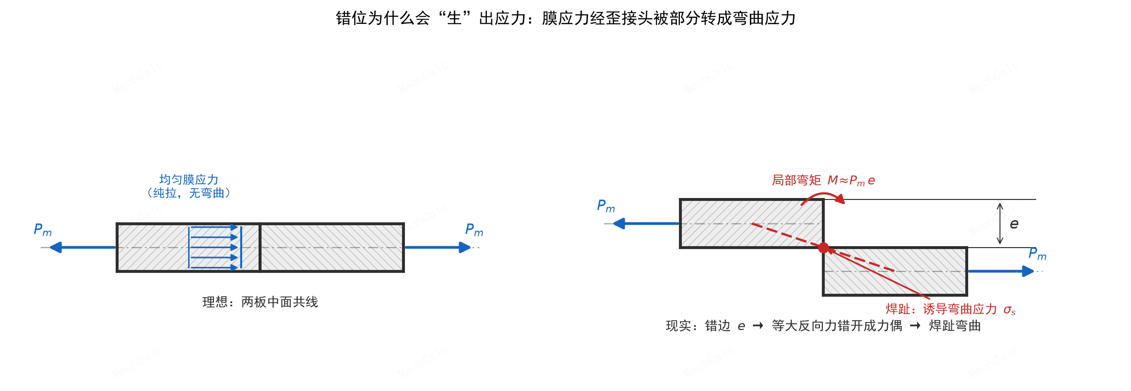
Figure 1: Why misalignment creates stress. Left — an ideal joint with the two neutral axes collinear; the end membrane forces are equal and opposite with coincident lines of action, and the section carries only uniform membrane stress. Right — a real joint offset by e; the end membrane forces are still equal and opposite (axial force balance) but their lines of action are offset by e, forming a couple M≈Pm·e that forces an induced bending stress σs at the weld toe (per BS 7910:2019, Annex D, D.1).
💡 The physics in one line: membrane stress (tension) passing through a “skewed joint” is partly converted into bending stress. This is the most typical engineering conversion between membrane and bending stress, and the product is a local bending stress at the weld toe.
1.2 Two basic misalignments + one special geometry
| Type | Symbol | Meaning |
|---|---|---|
| Axial misalignment (eccentricity) | $e$ | the two neutral axes are parallel but offset by $e$ |
| Angular misalignment | $\alpha$ (peaking $y$) | the two plates are joined at an angle $\alpha$, raising a ridge at the weld, with peaking $y$ |
| Ovality (special geometry) | $D_{max}-D_{min}$ | a pressure vessel or pipe is out of round and is “rounded out” under internal pressure, giving extra bending at the weld |
(BS 7910:2019, Annex D, D.0 + Table D.1)
1.3 Three applicability boundaries (easiest to get wrong)
- Directionality — $\sigma_s$ arises only under the membrane stress component $P_m$ perpendicular to the misalignment line; it does not arise from: ① a continuous weld loaded along its length; ② a plate in pure bending only. Exception: for a section or pipe under overall bending, its membrane stress component still re-generates extra bending through the misalignment.
- Sign — when several misalignments coexist, the total induced bending is the sum of each type; the same section has tension (+) / compression (−) at different through-thickness positions; the axial and angular components may add with the same sign, or cancel with opposite sign, so they must be added algebraically.
- Restraint — the amount of bending also depends on whether the joint can rotate freely under the induced moment (which depends on the load, boundary conditions, section shape and local reinforcement). Quantifying restraint usually needs finite element analysis; unless it can be shown that restraint reduces the effect, always compute as “unrestrained” (most conservative).
💡 Three shared conventions (remember before reading the formulas)
- Applies to butt and fillet joints; except for the fillet-weld root of the cruciform case (Table D.2 case c), all formulas give $\sigma_s$ at the weld toe.
- The formulas assume the shape deviation is measured under no load; if measured under load (e.g. a geometry gauge on a thin-wall pipe in service), correct it back to the no-load value.
- When assessing an embedded crack: the misalignment bending stress varies linearly through the thickness and is zero at the neutral axis; take the value at the crack depth from this distribution.
2. The core products: bending stress σs and magnification factor km
2.1 Two ways to use it + the definition of km
Every Annex D formula first gives the dimensionless ratio $\sigma_s/P_m$. With that ratio there are two routes: Route ① take $\sigma_s$ directly as the bending component into the fracture assessment; Route ② convert it to a magnification factor $k_m$:
$$k_m = \frac{P_m+\sigma_s}{P_m}=1+\frac{\sigma_s}{P_m} \qquad k_m = 1+\frac{\Delta\sigma_s}{\Delta P_m}\ \text{(stress-range form)}$$(BS 7910:2019, Annex D, Eq. D.1, D.2)
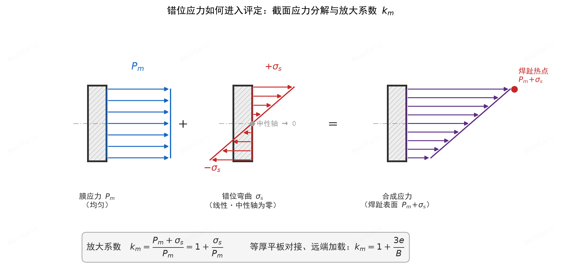
Figure 2: Stress decomposition at the weld section. Total stress = uniform membrane stress Pm + misalignment bending stress σs (linear through the thickness, zero at the neutral axis); combined, the weld-toe surface reaches a peak of Pm+σs, so the magnification factor km = (Pm+σs)/Pm = 1 + σs/Pm (per BS 7910:2019, Annex D, Eq. D.1).
2.2 Superposition of several misalignments
When axial and angular misalignment coexist, the magnification factors add linearly:
$$k_m = 1 + (k_m-1)_{\text{axial}} + (k_m-1)_{\text{angular}}$$(BS 7910:2019, Annex D, Eq. D.3; when superposing, mind the sign convention of §1.3 point 2 — same-sign addition may be more dangerous, opposite-sign may cancel)
2.3 A starting anchor: km = 1 + 3e/B
💡 One formula to get you started: equal-thickness plate butt joint, axial misalignment From Table D.1 case a, with unrestrained $\kappa=6$ and remote loading $l_1=l_2$, it simplifies to:
$$\frac{\sigma_s}{P_m}=\frac{3e}{B}\quad\Longrightarrow\quad k_m=1+\frac{3e}{B}$$The physics is clear at a glance: the larger the offset $e$ and the thinner the plate (smaller $B$), the stronger the magnification. Example: a 10 mm plate with a 2 mm offset gives $k_m=1.6$ — the membrane stress is magnified by 60%.
2.4 Primary or secondary stress?
The conservative choice is to treat it as primary stress (affecting both the vertical axis $K_r$ and the horizontal axis $L_r$); research shows that for girth-weld scenarios it can often be treated as secondary stress (affecting $K_r$ only, not $L_r$). Take primary first for safety, and relax to secondary when justified — a classic engineering case of the primary/secondary distinction.
2.5 Through-wall cracks: possibly over-conservative
The crack itself releases local bending — the longer the crack, the more it releases — so applying Annex D directly to a through-wall crack can be over-conservative; a dedicated analysis may be needed (BS 7910:2019, Annex D, D.1).
3. Table D.1: the 7 butt-joint types in detail
The common algorithm skeleton (each type follows these five steps): ① measure the geometry ($e$ or $\alpha,y$; and $B,l$ etc.) → ② choose the formula and parameters by configuration ($\kappa$, $n$, end condition) → ③ compute $\sigma_s/P_m$ → ④ get $\sigma_s=(\sigma_s/P_m)\,P_m$, $k_m=1+\sigma_s/P_m$ → ⑤ feed into the assessment (see Section 5).
a) Equal-thickness plate, axial misalignment
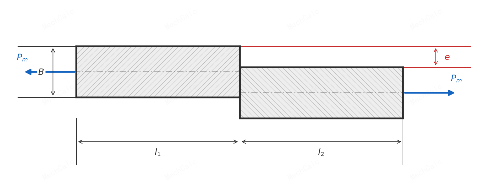
Figure 3a: Equal-thickness plate with axial misalignment e (per BS 7910:2019, Annex D, Table D.1 case a).
Algorithm: ① measure the offset $e$, plate thickness $B$, and the two spans $l_1,l_2$; ② take the restraint factor $\kappa$ — unrestrained take $\kappa=6$ (most conservative); ③ for remote loading set $l_1=l_2$, and the formula simplifies to $\sigma_s/P_m=3e/B$; ④ get $\sigma_s$ and $k_m=1+3e/B$.
(BS 7910:2019, Annex D, Table D.1 case a)
b) Unequal-thickness plate, axial misalignment ($B_2>B_1$)
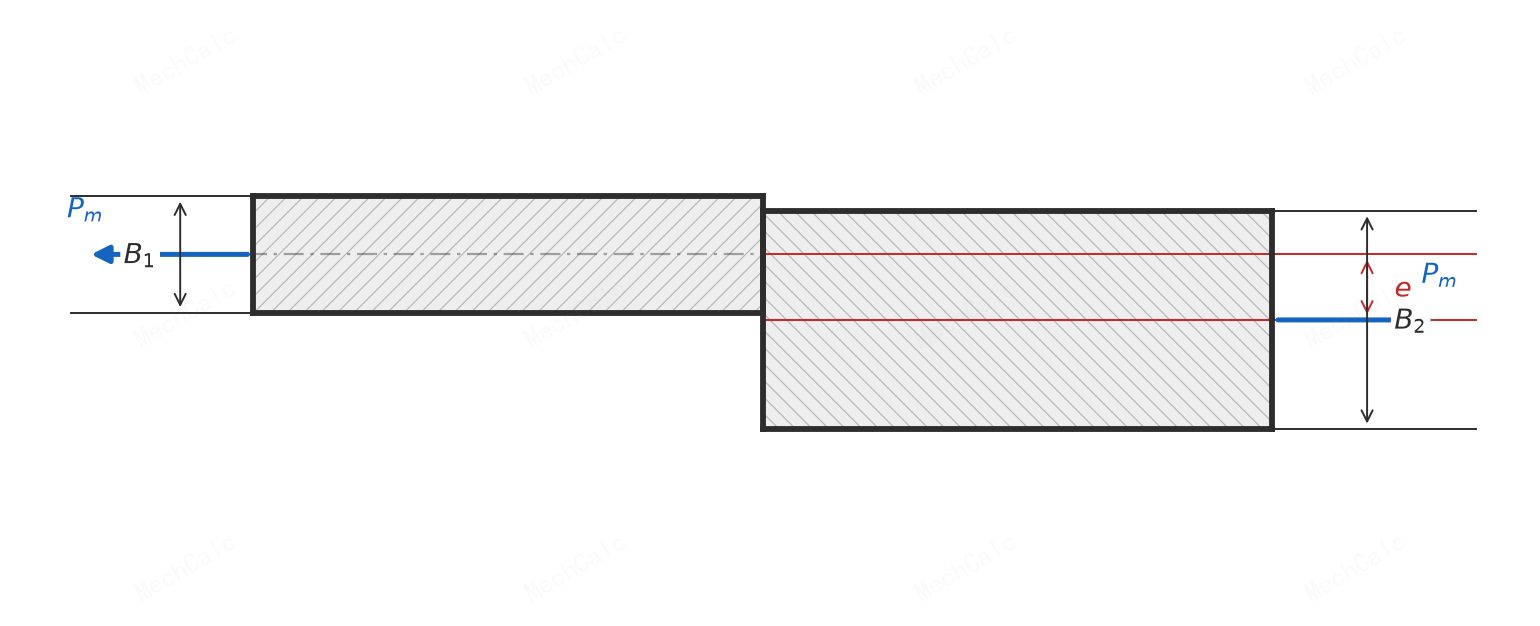
Figure 3b: Unequal-thickness plate with axial misalignment, B1 the thinner plate, B2 the thicker (per BS 7910:2019, Annex D, Table D.1 case b).
Algorithm: ① use the thinner plate $B_1$ as the reference; ② the thickness-ratio term $B_1^{\,n}/(B_1^{\,n}+B_2^{\,n})$ distributes the induced bending between the thin and thick plates by stiffness (the thick plate takes more, the thin plate’s weld-toe stress is reduced); ③ take $n=1.5$ (supported by tests); ④ applies to remote loading, unrestrained joints.
(BS 7910:2019, Annex D, Table D.1 case b)
c) Cylinder/pipe longitudinal weld, axial misalignment ($B_2\ge B_1$)
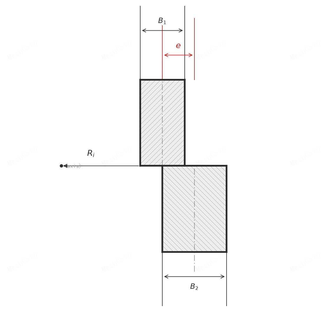
Figure 3c: Longitudinal weld of a cylinder or pipe with axial misalignment; on the cross-section there is a radial offset e at the longitudinal weld (per BS 7910:2019, Annex D, Table D.1 case c).
Algorithm: on top of the plate form, add two shell corrections — ① $(1-\nu^2)$ reflects the biaxial restraint of the shell wall (raising stiffness); ② the thickness ratio uses a power of 0.6. The rest of the flow is as in cases a, b.
(BS 7910:2019, Annex D, Table D.1 case c)
d) Cylinder/pipe girth weld + spherical-shell weld, axial misalignment ($B_2\ge B_1$)
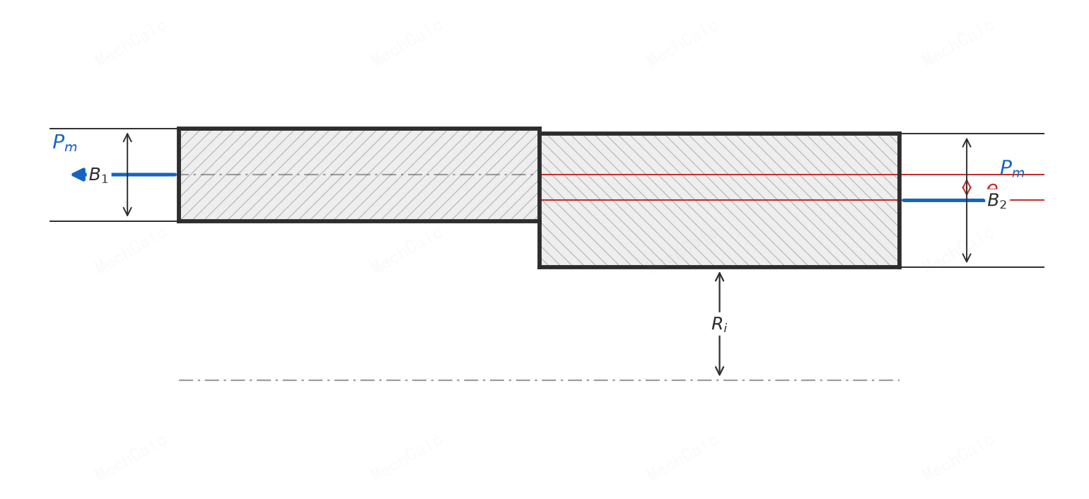
Figure 3d: Girth weld of a cylinder or pipe, and spherical-shell weld, with axial misalignment; axial section, with cylinder inner radius Ri (per BS 7910:2019, Annex D, Table D.1 case d).
The girth/spherical-shell weld uses a piecewise formula:
$$\sigma_s/P_m<1:\quad \frac{\sigma_s}{P_m}=\frac{6e}{B_1(1-\nu^2)}\left[\frac{1}{1+(B_2/B_1)^{1.5}}\right]$$$$\sigma_s/P_m\ge1:\quad \frac{\sigma_s}{P_m}=\frac{2.6e}{B_1}\left[\frac{1}{1+0.7(B_2/B_1)^{1.4}}\right]$$Algorithm: ① first try the first equation; ② if the result is $<1$ that is the final value; ③ if $\ge1$, recompute with the second equation (the two switch depending on whether $\sigma_s/P_m$ reaches 1).
(BS 7910:2019, Annex D, Table D.1 case d)
e) Plate, angular misalignment ($\alpha$ in radians)
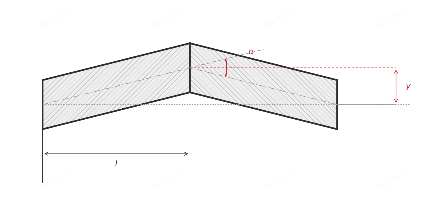
Figure 3e: Plate angular misalignment; α is the angle between the extension of the left plate’s neutral axis and the right plate’s neutral axis, with peaking y (per BS 7910:2019, Annex D, Table D.1 case e).
Fixed ends:
$$\frac{\sigma_s}{P_m}=\frac{3y}{B}\left[\frac{\tanh(\beta/2)}{\beta/2}\right]=\frac{3\alpha}{4}\frac{2l}{B}\left[\frac{\tanh(\beta/2)}{\beta/2}\right]$$Pinned ends:
$$\frac{\sigma_s}{P_m}=\frac{6y}{B}\left[\frac{\tanh\beta}{\beta}\right]=\frac{3\alpha}{2}\frac{2l}{B}\left[\frac{\tanh\beta}{\beta}\right],\qquad \beta=\frac{2l}{B}\sqrt{\frac{3\,\sigma_{max,m}}{E}}$$Algorithm: ① measure the angular distortion (peaking $y$ or angle $\alpha$, with $2l$ the span); ② choose the end condition (fixed or pinned) and take the matching equation; ③ compute $\beta$ (needs the maximum membrane stress $\sigma_{max,m}$ and the elastic modulus $E$); ④ the tanh correction — the bracket term is always $\le 1$, reflecting how tension “straightens” the angular distortion: under tension, ignoring it is conservative, and it can be ignored for $2l/B<10$; but under compression tanh becomes tan and cannot be ignored.
(BS 7910:2019, Annex D, Table D.1 case e)
f) Cylinder/vessel longitudinal or girth weld, angular misalignment
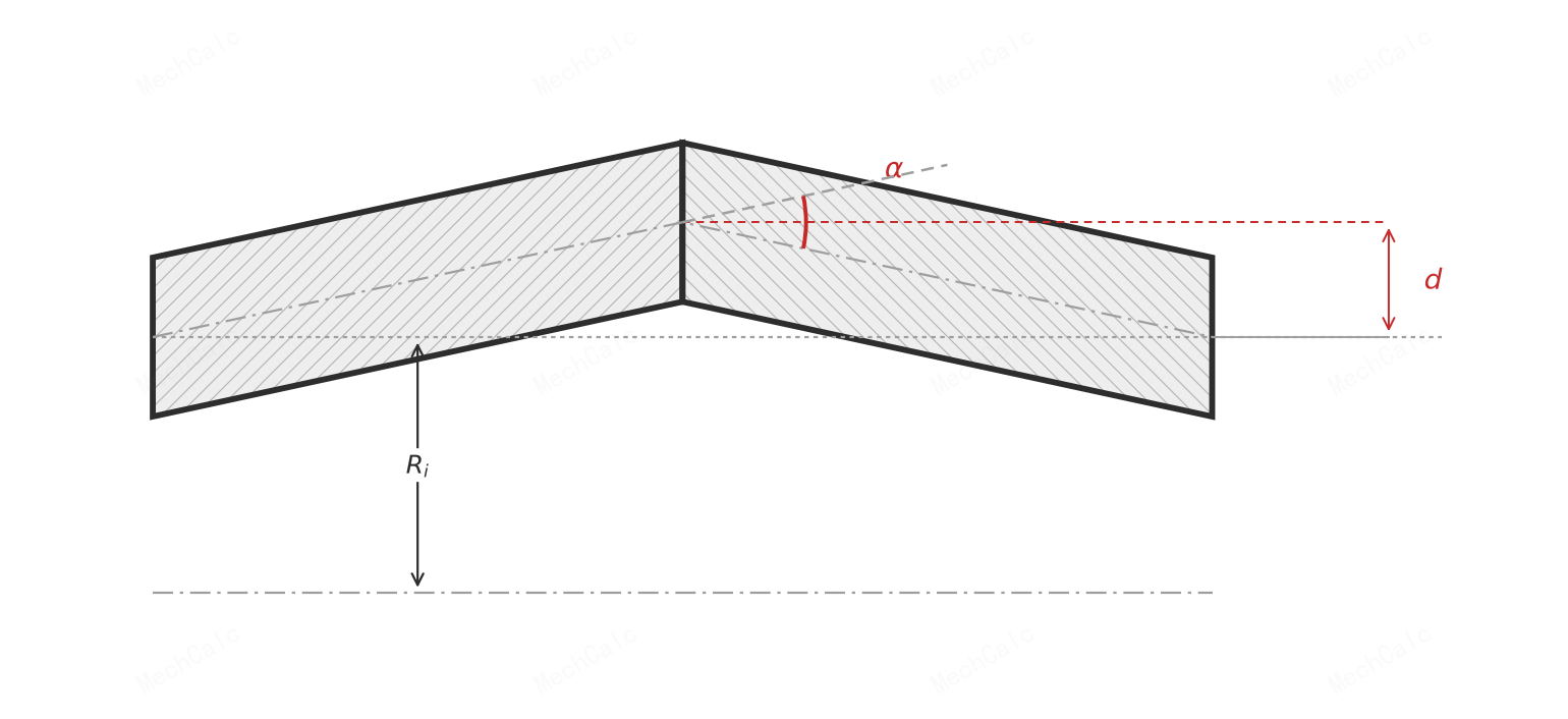
Figure 3f: Longitudinal or girth weld of a cylinder or vessel with angular misalignment; a fold in the curved wall, with inner radius Ri (per BS 7910:2019, Annex D, Table D.1 case f).
Fixed ends:
$$\frac{\sigma_s}{P_m}=\frac{3d}{B(1-\nu^2)}\left[\frac{\tanh(\beta/2)}{\beta/2}\right]$$Pinned ends:
$$\frac{\sigma_s}{P_m}=\frac{6d}{B(1-\nu^2)}\left[\frac{\tanh\beta}{\beta}\right],\qquad \beta=\frac{2l}{B}\sqrt{\frac{3(1-\nu^2)\,\sigma_{max,m}}{E}}$$Algorithm: as in case e, but ① use the deviation-from-round $d$ (for ideal geometry $d=y/2$ or $\alpha l/2$); ② add the shell restraint $(1-\nu^2)$ (which also enters $\beta$).
(BS 7910:2019, Annex D, Table D.1 case f)
g) Pressure pipe/vessel, ovality ($\theta$ in degrees)
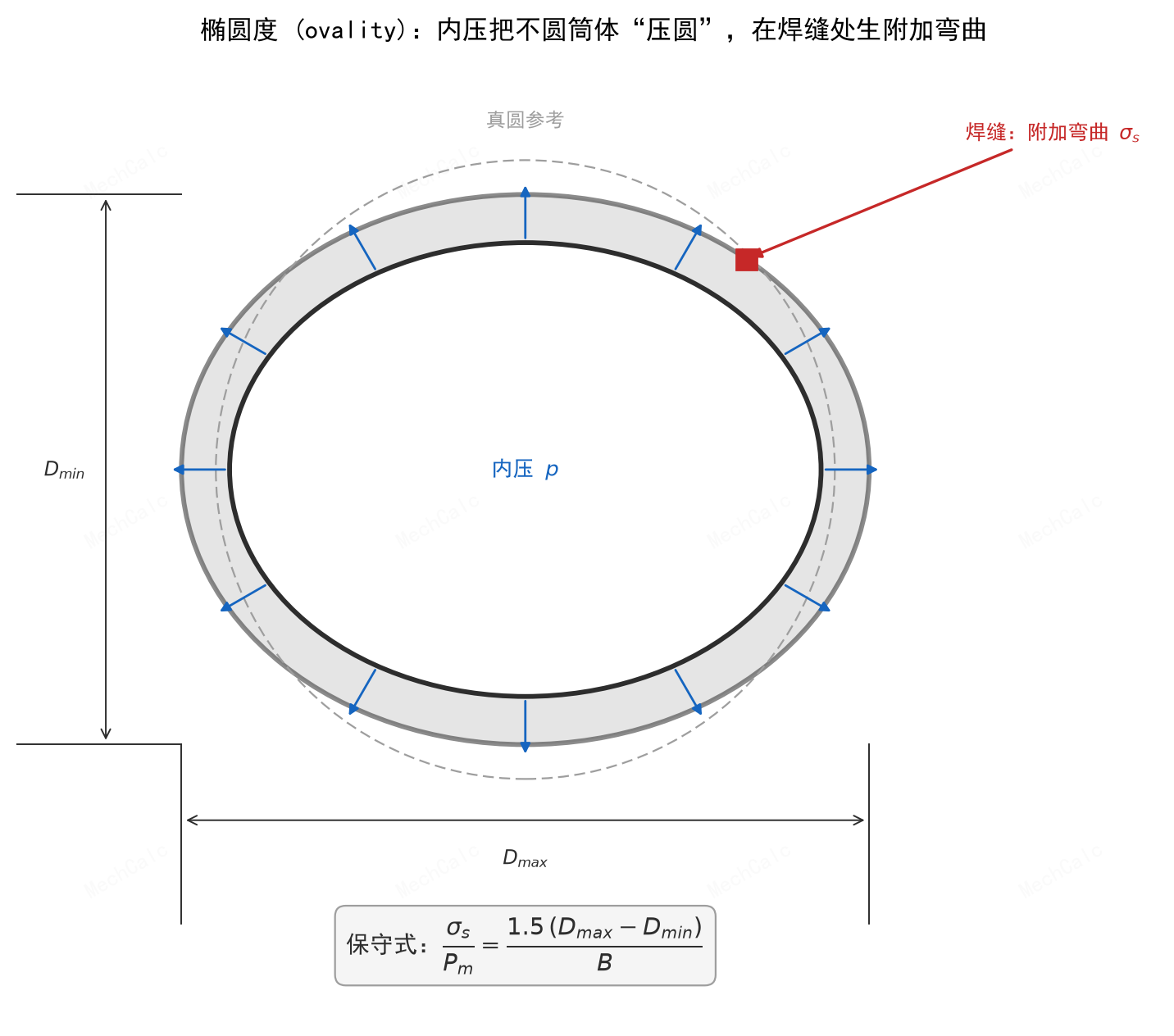
Figure 3g: Ovality of a pressure pipe or vessel, Dmax≠Dmin; internal pressure ‘rounds out’ the out-of-round section, producing extra bending stress at the weld (per BS 7910:2019, Annex D, Table D.1 case g).
Full form:
$$\frac{\sigma_s}{P_m}=\frac{1.5(D_{max}-D_{min})\cos 2\theta}{B\left\{1+0.5\left[\dfrac{p_m(1-\nu^2)}{E}\right]\left(\dfrac{D}{B}\right)^3\right\}}$$Conservative form:
$$\frac{\sigma_s}{P_m}=\frac{1.5(D_{max}-D_{min})}{B}$$Algorithm: ① measure the ovality $D_{max}-D_{min}$, the weld position angle $\theta$, and the internal pressure $p_m$; ② for a quick estimate use the conservative form; ③ for a precise value use the full form (which includes $\theta$ and the favourable reshaping by internal pressure “rounding out” the vessel — the denominator $\{\dots\}>1$, so $\sigma_s$ is reduced); ④ under fatigue loading with varying $p_m$, take the mean value over the period.
(BS 7910:2019, Annex D, Table D.1 case g)
4. Table D.2: the 3 cruciform / T-joint types in detail
The restraint parameter $\kappa$ in Table D.2 is not a single constant — it takes different values with the joint’s restraint and support (the original table gives values for several support sketches); representative values are listed below. The first two types concern fatigue failure at the parent-plate weld toe.
a) Butt or fillet weld, axial misalignment ($l_1\le l_2$)
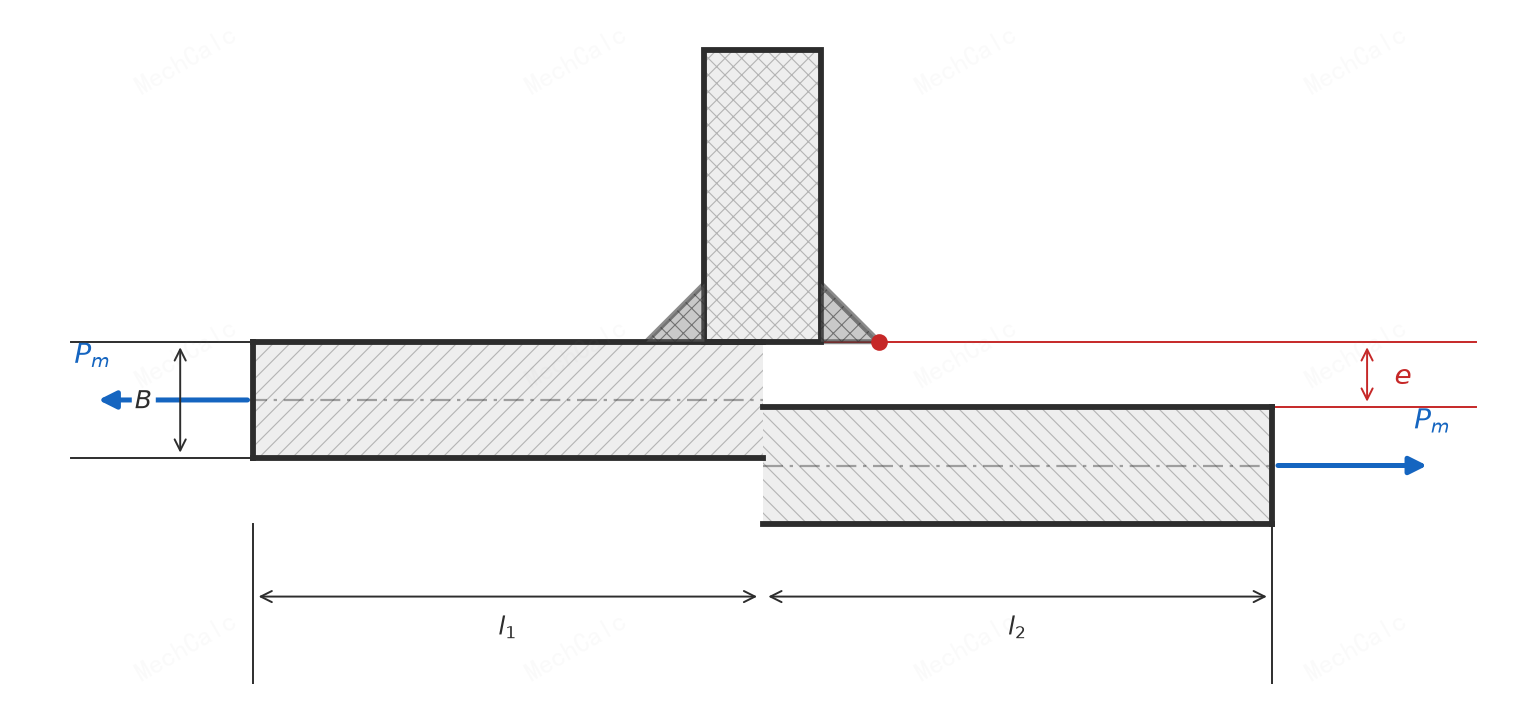
Figure 4a: Cruciform or T-joint butt or fillet weld with axial misalignment (per BS 7910:2019, Annex D, Table D.2 case a).
Algorithm: ① measure $e,B,l_1,l_2$; ② choose $\kappa$ by the actual restraint and support (the table’s representative values are $6.0 / 6.75 / 3.0 / 2.95$); ③ unrestrained with remote loading take $\kappa=6,\ l_1=l_2$; ④ get $\sigma_s$, $k_m$. Concerns fatigue failure at the parent-plate weld toe.
(BS 7910:2019, Annex D, Table D.2 case a)
b) Butt or fillet weld, angular misalignment
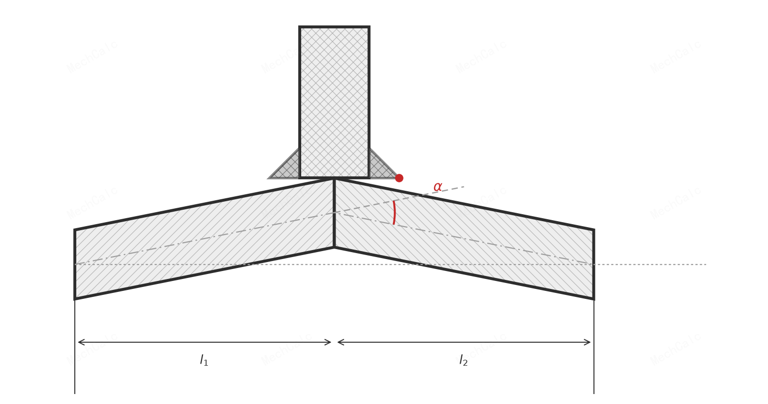
Figure 4b: Cruciform or T-joint butt or fillet weld with angular misalignment (per BS 7910:2019, Annex D, Table D.2 case b).
Algorithm: ① measure the angle $\alpha$ (radians), $B,l_1,l_2$; ② choose $\kappa$ by restraint (representative values $6.0 / 3.0 / 0.04 / 0.02$ — the restraint varies enormously, so take the value by the actual support, or the result may be off by two orders of magnitude); ③ get $\sigma_s$, $k_m$.
(BS 7910:2019, Annex D, Table D.2 case b)
c) Fillet weld, axial misalignment (failure through the weld throat/root)
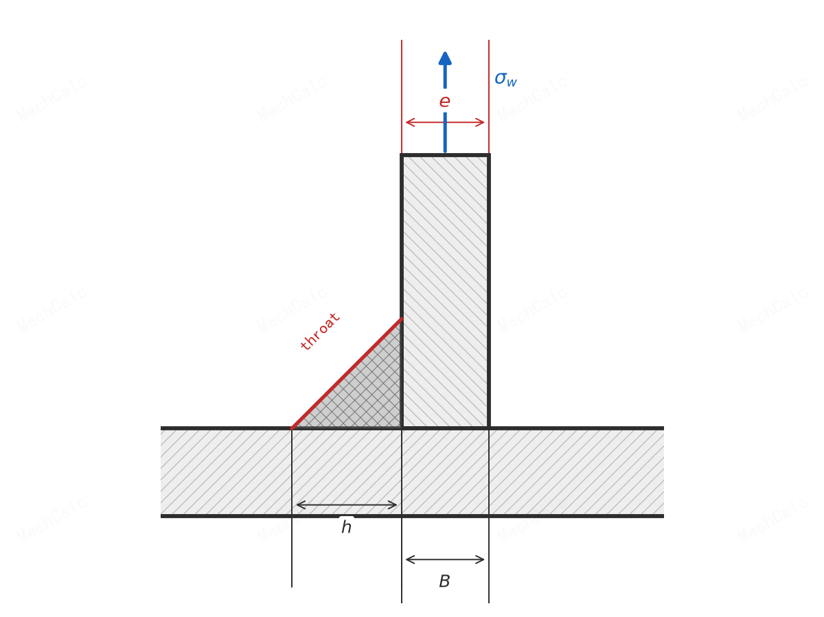
Figure 4c: Fillet weld with axial misalignment, the failure plane being the weld-throat inclined plane; σs/σw = e/(B+h), h the weld leg length (per BS 7910:2019, Annex D, Table D.2 case c).
Algorithm: ① note that this is referenced to the weld-throat stress $\sigma_w$ (not $P_m$); ② $h$ is the weld leg length; ③ concerns fatigue failure of the root through the weld throat.
⚠️ Two red lines
- Here the denominator is $B+h$ and the reference stress is $\sigma_w$ — do not mix it with the earlier formulas using $P_m$.
- This case cannot be used to compute the stress intensity factor of a weld-root flaw (BS 7910:2019, Annex D, Table D.2 case c).
5. After computing σs, which step of the assessment does it go into?
Annex D is not isolated — it supplies data to the main assessment (BS 7910:2019, 6.4.4).
5.1 Fracture assessment (FAD)
The misalignment bending stress $\sigma_s$, as a bending component, enters:
- the stress intensity factor $K_I$ calculation (Annex M);
- the reference stress $\sigma_{ref}$ calculation (Annex P).
Together they set the assessment point’s vertical coordinate $K_r$ and horizontal coordinate $L_r$ on the FAD; the primary/secondary choice is in §2.4.
5.2 Fatigue assessment (Clause 8)
- use $k_m$ to magnify the membrane stress range, adding the bending stress range $\Delta\sigma_s=(k_m-1)\Delta\sigma_m$ into the bending stress range (BS 7910:2019, 8.4);
- when misalignment is assessed on its own, judge with the $k_m$ acceptance limits of §8.8.1 and Table 8.10 (BS 7910:2019, 8.8.1, Table 8.10).
5.3 Value for an embedded crack
The misalignment bending stress varies linearly through the thickness and is zero at the neutral axis — when assessing an embedded flaw, take the value at the crack depth from this distribution (BS 7910:2019, Annex D, D.1).
6. Engineering pitfalls (recap)
- Directionality: $\sigma_s$ arises only under the membrane stress perpendicular to the misalignment line. Do not add this layer for a longitudinal continuous weld loaded lengthwise, or a pure-bending joint (§1.3 point 1).
- Compute restraint as unrestrained: unless restraint can be shown to reduce the effect, take $\kappa=6$ for plates (§1.3 point 3).
- Add signs algebraically: when axial + angular coexist they may add with the same sign (more dangerous) or cancel with opposite sign; add algebraically per Eq. D.3 (§2.2).
- The tanh correction is counter-intuitive: it can be ignored under tension (conservative); under compression it becomes tan and cannot be ignored (cases e, f).
- Cruciform $\kappa$ is not a fixed value: choose by the actual restraint, do not use the plate’s 6 (Table D.2 a, b).
- Fillet-weld case c uses $\sigma_w$ and cannot be used for the root SIF: do not mix it with $P_m$ or the weld-root stress intensity factor.
- Through-wall cracks may be over-conservative (§2.5).
Appendix: symbol quick reference
| Symbol | Meaning | Unit |
|---|---|---|
| $B$ / $B_1,B_2$ | section thickness / thickness of the two butt plates | mm |
| $D$ / $D_{max},D_{min}$ | mean diameter / maximum and minimum diameter | mm |
| $d$ | deviation from round caused by angular distortion | mm |
| $E$ | elastic modulus | N/mm² |
| $e$ | axial misalignment (eccentricity / centre-line offset) | mm |
| $h$ | weld leg length | mm |
| $k_m$ | misalignment stress magnification factor | — |
| $l$ / $l_1,l_2$ | distance from the misaligned joint to the load point or to the ends of the angular-distortion region (shortest is $l_1$) / plate length | mm |
| $n$ | factor for the bending-stress calculation of an unequal-thickness plate with axial misalignment | — |
| $P_m$ / $p_m$ | primary membrane stress / maximum pressure for the ovality calculation | N/mm² |
| $y$ | peaking caused by angular distortion | mm |
| $\alpha$ | angular change at the misalignment | radians |
| $\beta$ | factor for the angular-distortion bending-stress calculation | — |
| $\Delta P_m$ / $\Delta\sigma_s$ | primary membrane stress range / misalignment bending stress range | N/mm² |
| $\theta$ | angle between the weld and the point of maximum-diameter observation | ° |
| $\kappa$ | restraint parameter of the butt / cruciform joint | — |
| $\nu$ | Poisson’s ratio | — |
| $\sigma_{max,m}$ | membrane component of the maximum applied tensile stress | N/mm² |
| $\sigma_s$ | maximum induced bending stress due to misalignment (same sign as $P_m$) | N/mm² |
| $\sigma_w$ | applied stress on the weld throat | N/mm² |
(BS 7910:2019, Annex D, D.0)
Misalignment stress does not give a verdict by itself; it ultimately feeds into the fracture assessment. Take the computed $\sigma_s$ as the bending component, or multiply $k_m$ into the membrane stress, then run the Clause 7 Failure Assessment Diagram to reach the judgment of “whether the cracked structure may remain in service”.
🧮 在线计算器:BS 7910 Annex D Misalignment Stress Magnification k_m Calculator — Choose the misalignment geometry family, enter the geometry, and compute σs/Pm and the magnification factor km to feed into the Annex M stress intensity factor and the Clause 7 fracture assessment.
Figure note: Figures 1–4(c) are original MechCalc illustrations drawn from the BS 7910:2019 Annex D concepts and formulas, not copies of the standard’s figures.
📖 Reference:
- BS 7910:2019+A1:2020, Guide to methods for assessing the acceptability of flaws in metallic structures, Annex D — Stress due to misalignment