This is the first of four problems on the A533B-1 welded plate. The shared background, common method, and residual-stress profile for all four are set out in the overview post:
For the overview and method, see Where does residual stress push the assessment point? — A FAD recomputation of the A533B-1 large welded-plate fracture tests. This post focuses on one specimen and walks it through the calculator from input to reading the chart.
What this problem asks
LLAW = Low-$L_r$ + as-Welded: as-welded (no post-weld heat treatment), assessment temperature −120 ℃, low load ratio. Of the four specimens, it fractured at the lowest load (1.27 MN), with crack arrest afterwards. The low temperature drops the fracture toughness onto the lower shelf ($K_{mat}=37\ \mathrm{MPa\cdot m^{0.5}}$), while the full set of unrelaxed welding residual stresses still bears directly on the crack.
The aim here is to turn a qualitative statement — “welding residual stress is very damaging” — into a specific vertical-axis increment on the Failure Assessment Diagram (FAD).
The principle in brief: residual stress enters only $K_r$, not $L_r$
All four problems use the Option 1 (standard) Failure Assessment Diagram of BS 7910:2019 §7.3.3. The assessment-point coordinates:
$$ K_r = \frac{K_I^P + K_I^S}{K_{mat}} + \rho, \qquad L_r = \frac{\sigma_{ref}}{\sigma_Y} $$The Failure Assessment Line (FAL):
$$ f(L_r) = \begin{cases} \left(1 + \tfrac{1}{2}L_r^2\right)^{-1/2}\left[0.3 + 0.7\,e^{-\mu L_r^6}\right], & L_r \le 1 \\ f(L_r{=}1)\,L_r^{(N-1)/(2N)}, & 1 < L_r < L_{r,\max} \\ 0, & L_r \ge L_{r,\max} \end{cases} $$$$ \mu = \min\!\left(0.001\tfrac{E}{\sigma_Y},\ 0.6\right), \quad N = 0.3\left(1 - \tfrac{\sigma_Y}{\sigma_U}\right), \quad L_{r,\max} = \frac{\sigma_Y + \sigma_U}{2\sigma_Y} $$The three branches correspond to BS 7910:2019 §7.3.3 Eq. 7.26 ($L_r \le 1$, the brittle-fracture-governed branch), Eq. 7.27 ($1 < L_r < L_{r,\max}$, the elastic-plastic transition branch, where the curve bends down with the strain-hardening exponent $N$), and Eq. 7.28 ($L_r \ge L_{r,\max}$, plastic cut-off, where the curve drops to zero); the cut-off point $L_{r,\max}$ is given by Eq. 7.25. For this problem the assessment point sits at $L_r=0.367$, within the first branch, so the verdict below uses only Eq. 7.26.
The key engineering division of labour (BS 7910:2019, §7.3.6 / §7.3.7): welding residual stress is a secondary stress (a self-balancing field). It raises the vertical axis $K_r$ only and does not enter the horizontal axis $L_r$ — $L_r$ comes solely from the primary stress (here the bending stress of four-point bending), via the Annex P reference-stress solution. So the residual-stress contribution is simply the $K_I^S$ obtained by integrating the measured profile against the crack front with a weight function, entered directly and added into the numerator of $K_r$. For this problem the as-welded residual $K_I^S \approx 46\ \mathrm{MPa\cdot m^{0.5}}$.
Inputs at a glance
| Parameter | Value | Note |
|---|---|---|
| Flaw type | surface semi-elliptical (surface) | machined in the weld region |
| Crack depth $a_0$ / half-length $c_0$ | 19.4 / 87.5 mm | full length $2c_0=175$ mm |
| Plate thickness $B=t$ / width $W$ | 71 / 600 mm | |
| Primary membrane $P_m$ / bending $P_b$ | 0 / 245 MPa | pure bending (converted from the 1.27 MN fracture load) |
| Yield $\sigma_Y$ / tensile $\sigma_U$ | 618 / 791 MPa | base-metal properties |
| Elastic modulus $E$ | 210 GPa | |
| Fracture toughness $K_{mat}$ | 37 MPa·m$^{0.5}$ | as-welded weld @ −120 ℃, lower shelf |
| Residual $K_I^S$ (direct entry) | 46 MPa·m$^{0.5}$ | weight-function integration of the measured profile |
Entering it in the calculator
mechCalc’s Fracture Assessment Calculator groups the inputs into cards, and the very first card is the assessment option — choose the method first, then fill in the data:
- Assessment Option (FAD): pick Option 1 (Section 7.3.3) (it is the default).
- 1. Crack / Flaw Type: set geometry to
Flat Plateand flaw type toSurface semi-elliptical; enter crack depth 19.4 and half-length 87.5. - 2. Component Geometry: wall thickness 71, width 600.
- 3. Stress & Polynomial Coefficients: primary membrane stress $P_m=0$, primary bending $P_b=245$; for the secondary-load source choose
Enter $K_I^S$ directlyand enter $K_I^S=46$. - 5. Material: yield 618, tensile 791, modulus 210.
- 6. Fracture Toughness: source
Direct $K_{mat}$, enter 37. - 7. Analysis Type & Plasticity Interaction: leave the plasticity-interaction $\rho$ source at the default
Annex R (auto)— when a secondary stress is present, $\rho$ must be computed and cannot be set to zero, otherwise $K_r$ would be non-conservative.
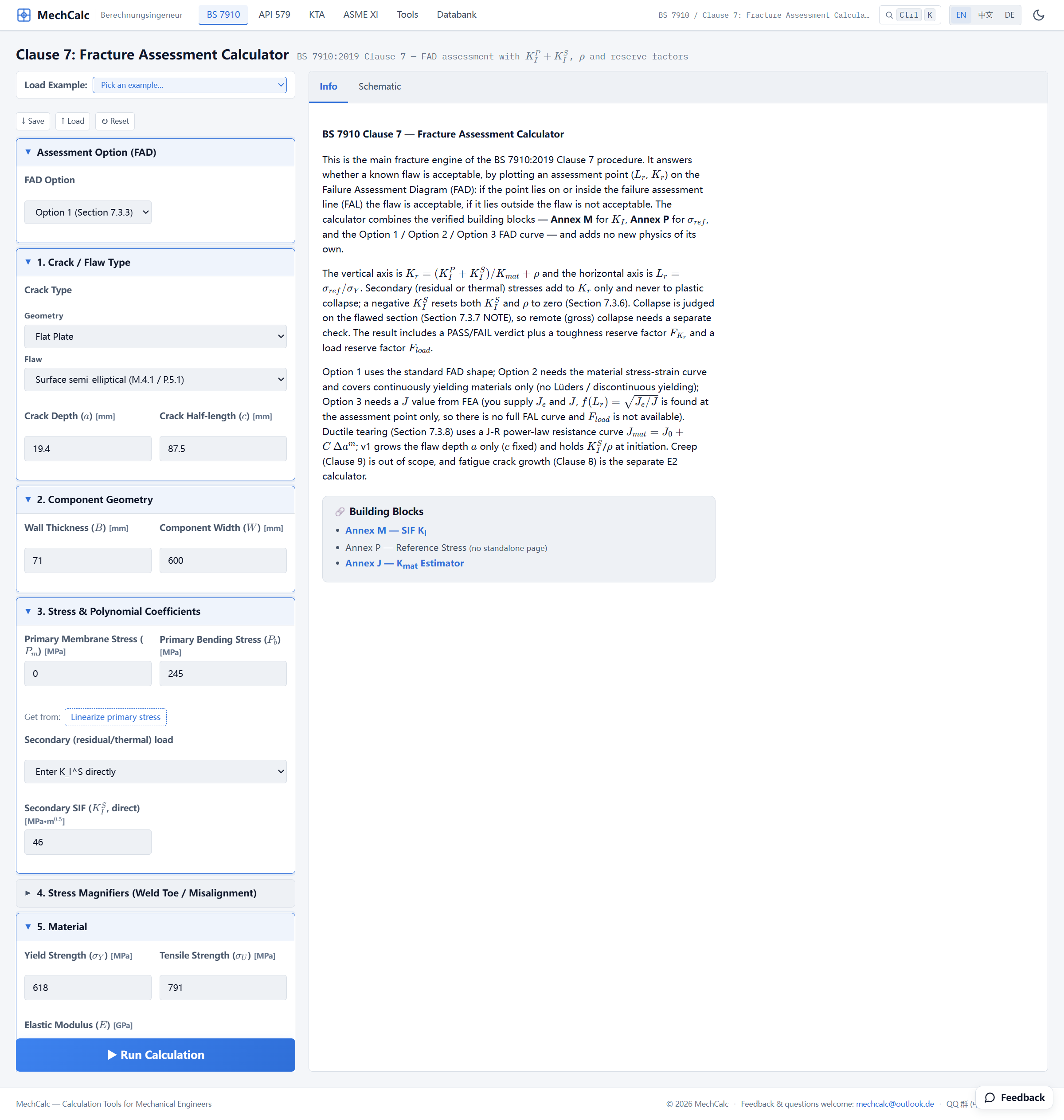
Figure 1: LLAW inputs in the BS 7910 Clause 7 Fracture Assessment Calculator. The top “Assessment Option (FAD)” already selects Option 1; the primary stress is bending only at 245 MPa, and the welding residual stress is entered directly through the secondary channel as K_I^S=46.
Once everything is filled in, click Run Calculation.
Results
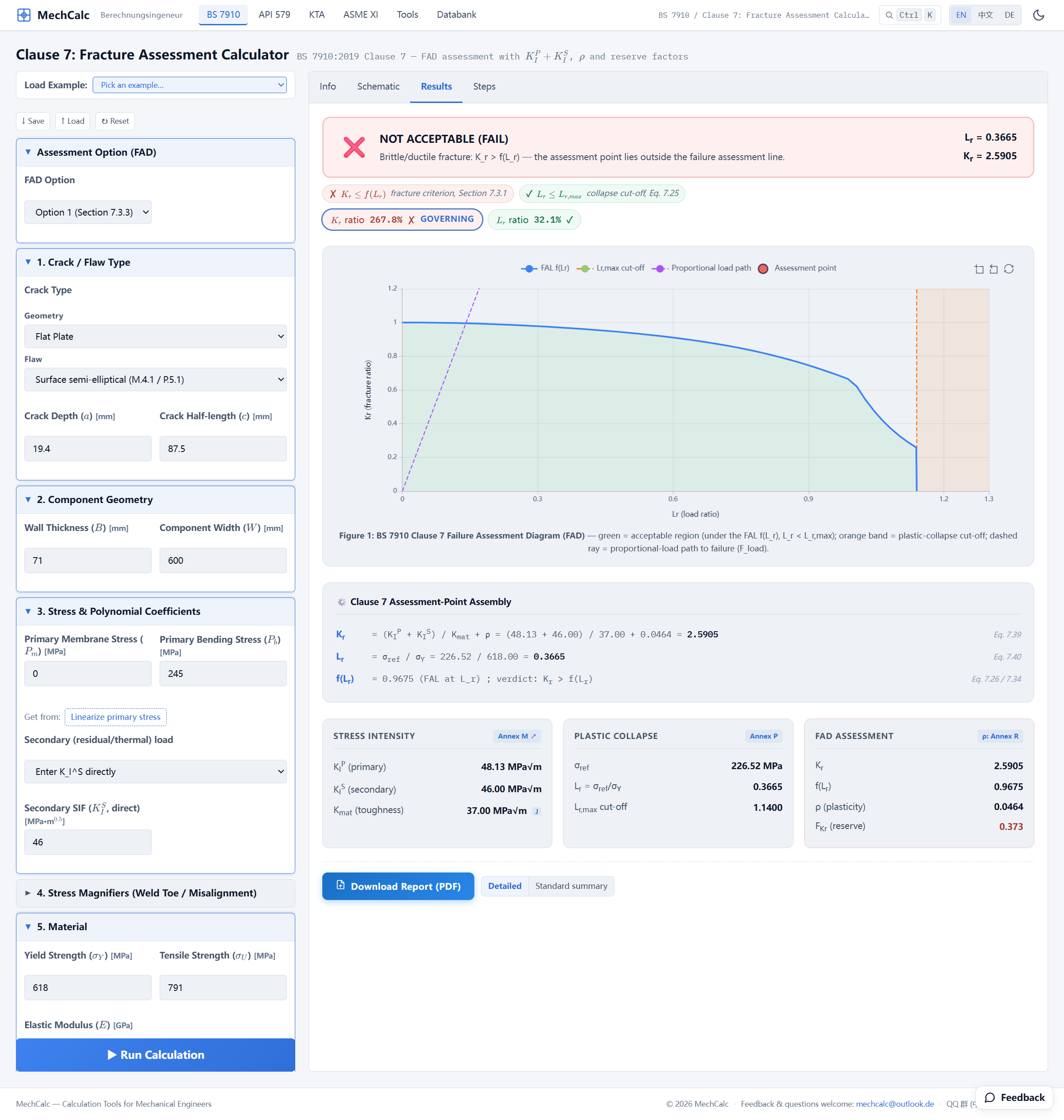
Figure 2: LLAW results. The assessment point (L_r, K_r)=(0.367, 2.59) lies far beyond the Failure Assessment Line, giving a verdict of NOT ACCEPTABLE. The three panels at lower right give the full set of intermediate quantities: K_I^p=48.13, K_I^s=46, σ_ref=226.5, ρ=0.046, f(L_r)=0.373.
The assessment point and intermediate quantities the engine assembles via the Clause 7 procedure:
| Quantity | Value | Source |
|---|---|---|
| Primary stress intensity factor $K_I^P$ | 48.13 MPa·m$^{0.5}$ | Annex M semi-elliptical surface-flaw solution |
| Secondary stress intensity factor $K_I^S$ | 46.00 MPa·m$^{0.5}$ | direct entry (integration of the measured profile) |
| Reference stress $\sigma_{ref}$ | 226.5 MPa | Annex P limit load |
| Plasticity interaction $\rho$ | 0.046 | Annex R |
| Horizontal coordinate $L_r$ | 0.367 | $\sigma_{ref}/\sigma_Y$ |
| Vertical coordinate $K_r$ | 2.59 | $(K_I^P+K_I^S)/K_{mat}+\rho$ |
| FAL height $f(L_r)$ | 0.373 | Eq. 7.26 |
| Verdict | not acceptable (brittle fracture governing) | $K_r \gg f(L_r)$ |
Reading the result
Break $K_r$ apart and it becomes obvious: the numerator $K_I^P + K_I^S = 48.13 + 46 = 94.13$, of which the residual-stress term alone accounts for nearly half. If this were a piece of base metal with no residual stress ($K_I^S=0$), $K_r$ would land near $48.13/37 \approx 1.30$; the welding residual stress pushes it to 2.59 — almost double.
The assessment point $(0.367,\ 2.59)$ lies far beyond the Failure Assessment Line (at the same horizontal coordinate the FAL is only $f(L_r)=0.373$), so the flawed structure is judged not acceptable. This matches the test exactly: LLAW fractured at the lowest load. The main force driving it past the critical line is precisely that residual stress intensity factor of 46 MPa·m$^{0.5}$.
Cross-check against FITNET: is mechCalc accurate?
The value of this problem is not only “getting a number” but checking mechCalc’s accuracy against the original literature result. Laying the two assessments side by side, term by term:
| Quantity | mechCalc | FITNET original | Difference |
|---|---|---|---|
| Primary $K_I^P$ [MPa·m$^{0.5}$] | 48.13 | ≈48 | ≈0 |
| Secondary $K_I^S$ [MPa·m$^{0.5}$] | 46.0 | 46 | same source |
| Load ratio $L_r$ | 0.367 | 0.36 | +1.9% |
| Fracture ratio $K_r$ | 2.59 | 2.58 | +0.4% |
In the low-$L_r$, brittle-fracture-governed region — the very range that matters most to this test series — the two implementations agree almost digit for digit: $K_r$ differs by only 0.4% and $L_r$ by 1.9%. Bear in mind that the primary SIF and limit load on each side come from different analytical solutions (FITNET uses Sharples & Clayton / Sattari-Far, mechCalc uses BS 7910 Annex M / Annex P), and only the residual $K_I^S$ is taken from the same measured profile. Agreement this close is enough to show that mechCalc assembles correctly and gives trustworthy numbers at the residual-stress step — the one most prone to error.
Source: the FITNET project’s Case Studies for Fracture, case “A533B-1 Steel Residual Stress Experiments”; original test report C C France, J K Sharples & C Wignall, AEA Technology Report AEAT-4236 (SINTAP/TASK4/AEAT18, 1998).
Next problem preview: same temperature, same region, same measured residual profile — the only variable is that post-weld heat treatment (PWHT) was applied, dropping the residual $K_I^S$ from 46 to 5. How far does the assessment point fall back? See Problem 2 LLHT.
🧮 在线计算器:BS 7910 Clause 7 Fracture Assessment Calculator — Re-run this problem yourself: pick Option 1, enter the inputs from the table above, enter the secondary stress directly as K_I^S=46, and you get L_r=0.367, K_r=2.59.