In the FAD assessment of the four A533B welded-plate problems, the residual stress intensity factor for the as-welded case, $K_I^S \approx 46\ \mathrm{MPa\cdot m^{0.5}}$, has always been entered directly: FITNET obtained it by integrating the measured residual stress profile, and we simply fed that ready-made number into the vertical coordinate $K_r$.
A natural follow-up question: how does that 46 actually emerge from a residual stress curve, and can mechCalc compute it on its own?
It can. This is exactly what the BS 7910 Annex M.4.2 solution (finite-plate surface flaw, polynomial stress) does: given a stress polynomial $\sigma(x)$ distributed through the wall thickness, it integrates that stress along the crack front with a weight function to obtain the stress intensity factor of the crack. In this post we run that single step with the Annex M calculator in mechCalc, integrating the as-welded residual profile into the deepest-point SIF, and then compare it with the 46 from FITNET. This is a pure single-point stress intensity factor calculation, independent of any FAD assessment.
Principle: polynomial stress profile → SIF
The flaw being assessed is a semi-elliptical surface crack in the weld region (depth $a$, surface half-length $c$). The secondary stress (welding residual) is not constant through the wall thickness but follows a curve, which BS 7910 describes with a polynomial of degree up to five (the coordinate $x$ is measured from the cracked surface and normalised by the wall thickness $B$):
$$ \sigma(x) = \sum_{n=0}^{5} \sigma_n \left(\frac{x}{B}\right)^n $$The deepest-point $K_I$ is assembled per Eq. M.13 of Annex M.4.2.2: each stress order is paired with a Fett geometry function $f_i^d$ (read from Table M.1, with bilinear interpolation over $a/B$ and $a/2c$), and the sum is multiplied by $\sqrt{\pi a}$:
$$ K_I = \sqrt{\pi a}\,\sum_{i=0}^{5} \sigma_i \left(\frac{a}{B}\right)^{i} f_i^{\,d}\!\left(\frac{a}{B},\ \frac{a}{2c}\right) $$Source: BS 7910:2019, Annex M.4.2.2, Eq. M.13, Table M.1 (deepest point) / Table M.2 (surface point); geometry functions taken from Fett & Munz (1997) [M.10] and Fett, Munz & Neumann (1990) [M.11].
The key point: this solution’s polynomial convention is precisely $\sigma_n(x/B)^n$ (normalised by wall thickness, $x$ measured from the cracked surface). The A533B measured residual profile is already given in terms of $x/t$ (with $t=B$), so the coefficients map term by term with no change of variable needed.
Inputs: the A533B as-welded residual profile
The as-welded (LLAW / HLAW) measured residual stress profile given in §2.2 of the overview post (transverse to the weld, for the $x/t \le 0.5$ range, which covers $a/t=0.273$):
$$ \sigma^*(x/t) = -108.35 + 3543.6\,(x/t) - 9871.5\,(x/t)^2 + 2930.3\,(x/t)^3 \quad [\mathrm{MPa}] $$Mapping each term onto the Annex M.4.2 polynomial coefficients, and taking the crack and plate geometry of the LLAW as-welded specimen:
| Parameter | Value | Note |
|---|---|---|
| Crack depth $a$ | 19.4 mm | LLAW as-welded pre-crack depth |
| Crack surface half-length $c$ | 87.5 mm | Full length $2c = 175$ mm |
| Plate thickness $B = t$ | 71 mm | $a/B = 0.273$, within the Fett table grid |
| Section width $W$ | 600 mm | Finite-width correction |
| $\sigma_0$ | −108.35 MPa | Surface ($x=0$) residual stress, compressive |
| $\sigma_1$ | 3543.6 MPa | First-order term |
| $\sigma_2$ | −9871.5 MPa | Second-order term |
| $\sigma_3$ | 2930.3 MPa | Third-order term |
| $\sigma_4,\ \sigma_5$ | 0 | The profile is a cubic polynomial |
Entering it in the calculator
Open the BS 7910 Annex M stress intensity factor calculator in mechCalc and set it up in three steps:
- Geometry Group: choose Flat Plate.
- Flaw Type: choose M.4.2 · Finite Surface Polynomial [Fett] — this is the finite surface flaw solution under a polynomial stress profile.
- Enter the geometry and polynomial coefficients: crack depth 19.4, surface half-length 87.5; plate thickness 71, section width 600; polynomial $\sigma_0..\sigma_3$ as in the table above ($\sigma_4=\sigma_5=0$).
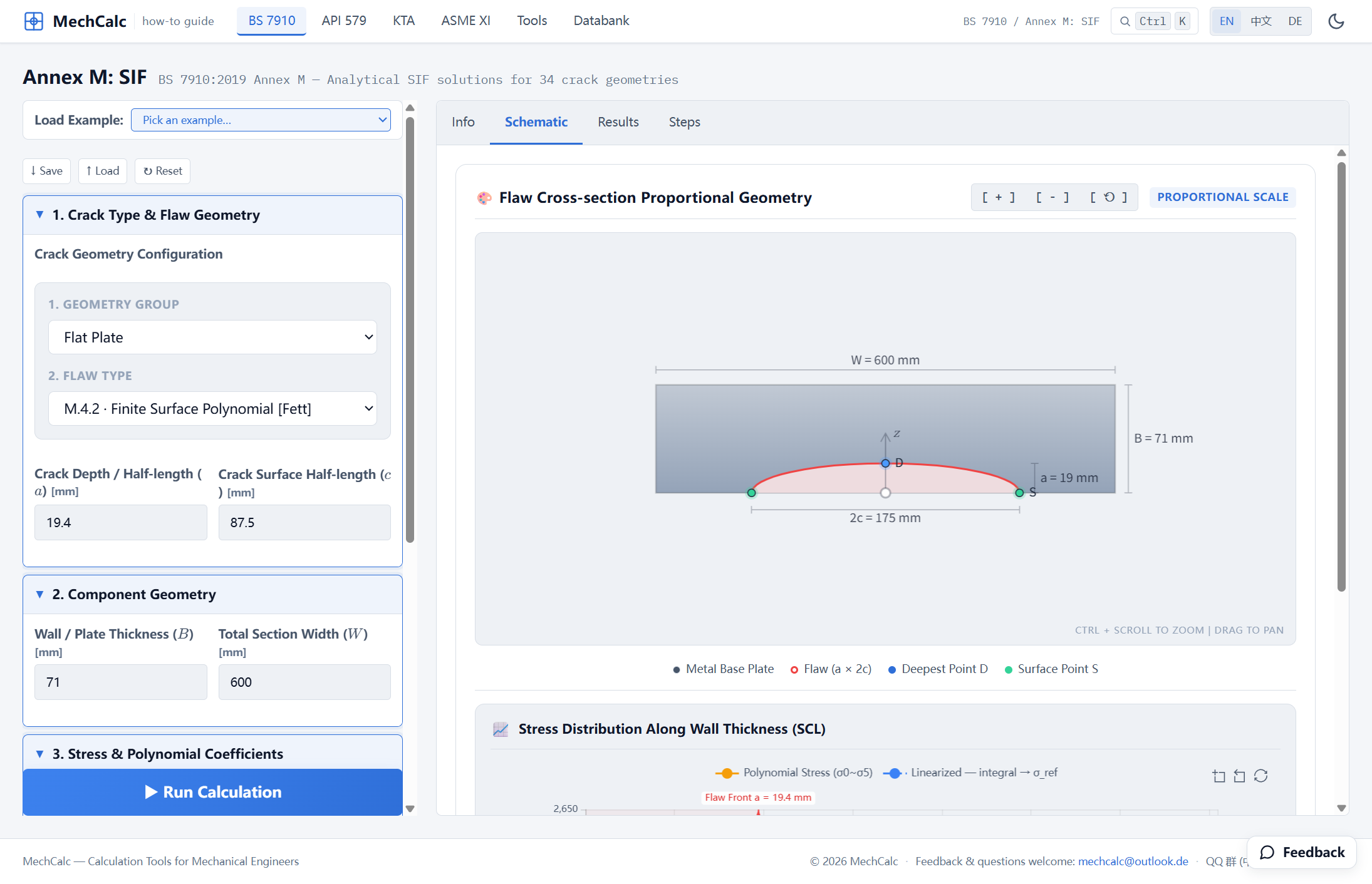
Figure 1: Selecting M.4.2 (finite-plate surface flaw, polynomial stress) in the Annex M calculator and entering the A533B as-welded residual stress polynomial. The ‘Flaw Cross-section Proportional Geometry’ panel on the right draws the crack to scale: a semi-elliptical surface crack (red) of depth a=19.4 mm and full length 2c=175 mm on a W=600 mm wide plate, with the deepest point D and surface point S marked.
The calculator also draws this residual stress distribution through the wall thickness in real time and to scale — this is exactly the quantity being integrated:
![Figure 2: Residual stress distribution through the wall thickness (orange line, polynomial σ₀~σ₅). The surface (x=0) is in compression at −108 MPa, turns rapidly to tension with depth, and peaks in the mid-thickness region; the dashed red vertical line marks the crack-front position at a=19.4 mm. The dashed blue line is the linearised equivalent (membrane + bending). The deepest-point K_I is the result of integrating this curve over [0, a] along the crack front with the weight function.](annexm-stress.png)
Figure 2: Residual stress distribution through the wall thickness (orange line, polynomial σ₀~σ₅). The surface (x=0) is in compression at −108 MPa, turns rapidly to tension with depth, and peaks in the mid-thickness region; the dashed red vertical line marks the crack-front position at a=19.4 mm. The dashed blue line is the linearised equivalent (membrane + bending). The deepest-point K_I is the result of integrating this curve over [0, a] along the crack front with the weight function.
Results
Click Run Calculation to obtain the SIF at the two crack-front points:
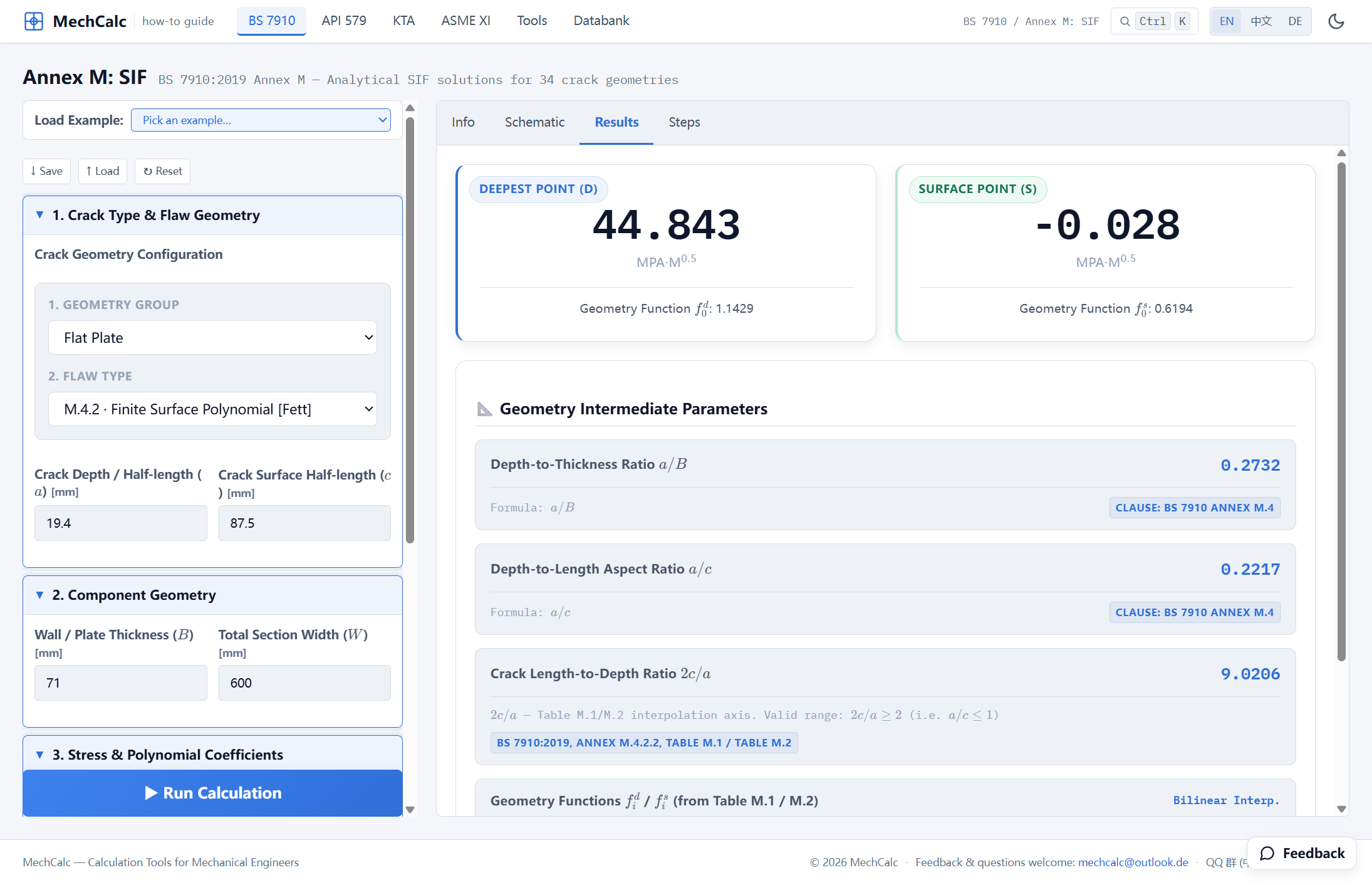
Figure 3: Annex M.4.2 results. Deepest point D: K_I = 44.843 MPa·m^0.5 (geometry function f₀ᵈ=1.1429); surface point S: K_I ≈ −0.028 ≈ 0. Below are the intermediate quantities a/B=0.2732, a/c=0.2217, 2c/a=9.0206, with the source cited as BS 7910 Annex M.4.2.2 Table M.1/M.2.
| Crack-front point | $K_I$ [MPa·m$^{0.5}$] | Note |
|---|---|---|
| Deepest point D | 44.843 | The residual $K_I^S$ that enters the FAD |
| Surface point S | −0.028 (≈ 0) | Near-surface compression, net contribution almost zero |
Why is the surface point almost zero? The surface-point geometry function weights the near-surface region most heavily, and there the residual stress is compressive (−108 MPa at $x=0$); compressive stress contributes negatively to the opening-mode SIF and just cancels the small amount of tension in the shallow layer, leaving net $K_I \approx 0$. The deepest point, by contrast, sees the large band of tension in the mid-thickness region, and so integrates out to 44.8 MPa·m$^{0.5}$ — this is the residual $K_I^S$ the assessment needs.
Whitebox: term-by-term expansion of Eq. M.13
The Whitebox steps in the calculator lay out the deepest-point summation in full ($a=0.0194$ m):
$$ K_I = \sqrt{\pi a}\,\big[\underbrace{-108.35{\times}1.0000{\times}1.1429}_{\sigma_0\text{ term}} + \underbrace{3543.6{\times}0.2732{\times}0.6585}_{\sigma_1\text{ term}} + \underbrace{-9871.5{\times}0.0747{\times}0.4820}_{\sigma_2\text{ term}} + \underbrace{2930.3{\times}0.0204{\times}0.3873}_{\sigma_3\text{ term}}\big] = 44.84 $$Here the Fett geometry functions (Table M.1, deepest point), obtained by bilinear interpolation at $a/B=0.273$ and $2c/a=9.02$, are $f_0^d{=}1.1429,\ f_1^d{=}0.6585,\ f_2^d{=}0.4820,\ f_3^d{=}0.3873$. Every step traces back to a table in the standard — no black box.
Cross-check against FITNET: is mechCalc accurate?
Placing the residual $K_I^S$ that mechCalc computed independently alongside the value reported by FITNET:
| Quantity | mechCalc (Annex M.4.2) | FITNET | Difference |
|---|---|---|---|
| Deepest-point residual $K_I^S$ [MPa·m$^{0.5}$] | 44.84 | ≈ 46 | −2.5% |
A 2.5% difference — for a cross-method check, that is very good agreement. Both sides do the same thing, “integrate the same measured residual profile along the crack front with a weight function”, but they use different weight function solutions: mechCalc uses the Fett tabulated geometry functions of BS 7910 Annex M.4.2, while FITNET uses the weight function solution built into its own procedure. For the same physical quantity computed by different methods, a difference of a few percent is normal, and here mechCalc comes out slightly lower (closer to the data, not overshooting).
What matters here is this: that “given out of nowhere” $K_I^S=46$ in the four-problem FAD assessment can be reproduced independently by mechCalc, from the raw residual stress profile, to within −2.5%, using its own Annex M.4.2 solution. In other words, residual stress — the most error-prone intermediate step — does not require mechCalc to take a fed value from the literature; it closes the loop on its own, and the result is confirmed by a third-party source.
Methodological note (DIFF is not FAIL): this comparison is the “self-generated” path check for $K_I^S$ in the four residual stress problems — a −2.5% difference between two weight function solutions for the same physical quantity is a normal methodological difference, already quantified and explained, and mechCalc holds up. For methodological cleanliness, the four FAD problems still consistently use the direct $K_I^S$ value from the same FITNET source.
Source: the FITNET project’s Case Studies for Fracture, case “A533B-1 Steel Residual Stress Experiments”; original test report C C France, J K Sharples & C Wignall, AEA Technology Report AEAT-4236 (SINTAP/TASK4/AEAT18, 1998). The SIF solution follows BS 7910:2019+A1:2020, Annex M.4.2.2 (Eq. M.13, Table M.1/M.2).
🧮 在线计算器:BS 7910 Annex M Stress Intensity Factor Calculator — Run it yourself: set Geometry Group to Flat Plate, Flaw Type to M.4.2 (Finite Surface Polynomial), enter a=19.4, c=87.5, B=71, W=600, and the polynomial σ₀=−108.35, σ₁=3543.6, σ₂=−9871.5, σ₃=2930.3 to obtain the deepest-point K_I=44.84 MPa·m^0.5.